Chapter 32 Two-way ANOVA Completely Randomized
library(tidyverse)
library(ez)
library(knitr)
library(kableExtra)
library(viridis)
library(DescTools)
A two-way ANOVA experimental design is one that involves two predictor variables, where each predictor has 2 or more levels. There is only one outcome variable in a 2 way ANOVA and it is measured on an equal interval scale. The predictor variables are often referred to as factors, and so ANOVA designs are synonymous with factorial designs.
The experimental designs can be as follows:
- Completely randomized (CR) on both factors
- Related measures (RM) on both factors
- Mixed, CR on one factor and RM on the other
In one sense, a two-way ANOVA can be thought of as two one-way ANOVA’s run simultaneously. The major difference, however, is the ability to test whether an interaction exists between the two factors.
In this chapter we’ll focus on the data structure and analysis of a two-way ANOVA CR experimental design.
32.1 Effect of Strain and Diet on Liver
A (hypothetical) study was conducted to evaluate the influence of mouse background strain and diet on the accumulation of cholesterol in liver. Ten animals were selected randomly from each of the C57BL/6 and C57BL/10 strains. They were each split randomly onto either of two diets, normal and high fat.
After about two months they were sacrificed to obtain cholesterol measurements in liver tissue.
Three predictions, and the corresponding null hypotheses that each tests, can be evaluated here simultaneously:
- The two strains differ in liver cholesterol content. \(H0:\sigma^2_{strain}\le\sigma^2_{residual}\)
- The diets differ in how they affect liver cholesterol content. \(H0:\sigma^2_{diet}\le\sigma^2_{residual}\)
- The liver cholesterol content is influenced by both diet and strain. \(H0:\sigma^2_{strainXdiet}\le\sigma^2_{residual}\)
The first two of these are commonly referred to as the main effects of the factors, whereas the third is referred to as the interaction effect of the factors.
Here’s some simulated data. But they are guided guided using means and standard deviations from the Jackson Labs phenome database). along with a graph of the results:
| ID | Strain | Diet | Cholesterol |
|---|---|---|---|
| 1 | C57BL/6 | Normal | 49 |
| 2 | C57BL/6 | Normal | 43 |
| 3 | C57BL/6 | Normal | 44 |
| 4 | C57BL/6 | Normal | 37 |
| 5 | C57BL/6 | Normal | 47 |
| 6 | C57BL/6 | High Fat | 91 |
| 7 | C57BL/6 | High Fat | 86 |
| 8 | C57BL/6 | High Fat | 120 |
| 9 | C57BL/6 | High Fat | 111 |
| 10 | C57BL/6 | High Fat | 101 |
| 11 | C57BL/10 | Normal | 100 |
| 12 | C57BL/10 | Normal | 123 |
| 13 | C57BL/10 | Normal | 125 |
| 14 | C57BL/10 | Normal | 115 |
| 15 | C57BL/10 | Normal | 88 |
| 16 | C57BL/10 | High Fat | 207 |
| 17 | C57BL/10 | High Fat | 228 |
| 18 | C57BL/10 | High Fat | 217 |
| 19 | C57BL/10 | High Fat | 220 |
| 20 | C57BL/10 | High Fat | 217 |
ggplot(
  liver,
  aes(Diet, Cholesterol, fill=Strain)
  ) +
  stat_summary(
    fun.data="mean_sdl",
    fun.args=list(mult=1),
    geom= "errorbar",
    position=position_dodge(width=1),
    width=0.2,
    size=1
    ) +
   stat_summary(
     fun.y="mean",
     fun.args=list(mult=1),
     geom= "bar",
     position=position_dodge(width=1),
     width=0.5,
     size=2
     ) +
  scale_fill_viridis(
    discrete=T
    ) +
  theme(
    legend.position=(c(0.8, 0.8))
    ) +
  labs(
    title="Strain and Diet Effects on Liver Cholesterol, mean +/- SD",
    x="Diet",
    y="Liver Cholesterol, mg/"
    )
## Warning: `fun.y` is deprecated. Use `fun` instead.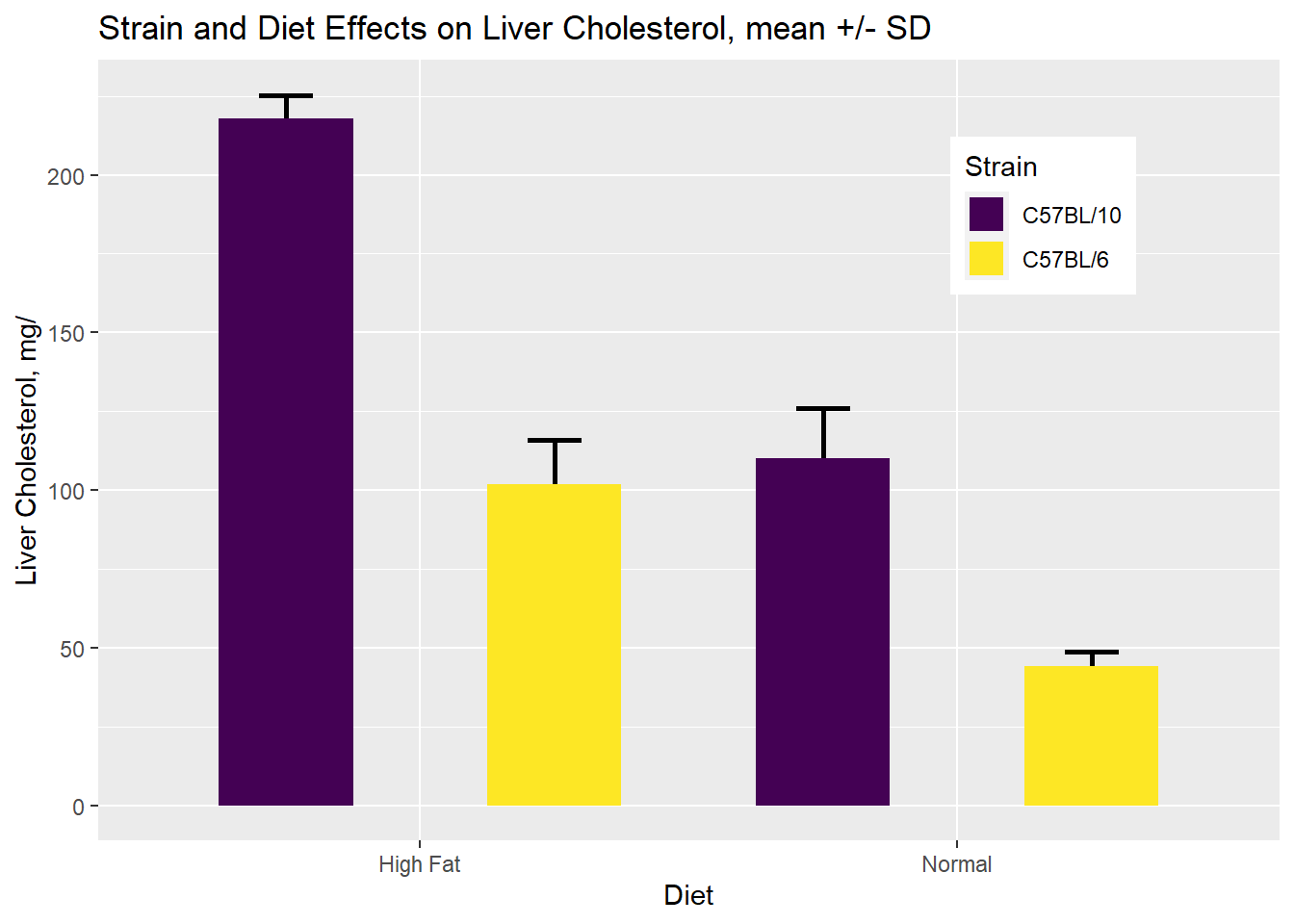
Figure 32.1: Two-way completely randomized ANOVA results
In particular, pay attention to the data structure. It has four columns: ID, Strain, Diet, Cholesterol. All of these are variables, including two columns for each of the predictor variables (Strain, Diet), and one for the response variable (Cholesterol). The ID can also be thought of as a variable.
32.2 The test
We use ezANOVA in the ANOVA package to test the three null hypotheses. Here are the arguments:
out.cr <- ezANOVA(data = liver,
                   dv = Cholesterol,
                   wid = ID,
                   between = c(Strain,Diet),
                   type = 3,
                   return_aov = T,
                   detailed = T

)

out.cr
## $ANOVA
## Effect DFn DFd SSn SSd F p p<.05 ges
## 1 (Intercept) 1 16 280608.05 2096.4 2141.63747 1.801635e-18 * 0.9925845
## 2 Strain 1 16 41496.05 2096.4 316.70330 5.742386e-12 * 0.9519091
## 3 Diet 1 16 34196.45 2096.4 260.99180 2.499051e-11 * 0.9422366
## 4 Strain:Diet 1 16 3100.05 2096.4 23.65999 1.722945e-04 * 0.5965707
##
## $`Levene's Test for Homogeneity of Variance`
## DFn DFd SSn SSd F p p<.05
## 1 3 16 283.8 748.4 2.022448 0.1513253
##
## $aov
## Call:
## aov(formula = formula(aov_formula), data = data)
##
## Terms:
## Strain Diet Strain:Diet Residuals
## Sum of Squares 41496.05 34196.45 3100.05 2096.40
## Deg. of Freedom 1 1 1 16
##
## Residual standard error: 11.44662
## Estimated effects may be unbalanced32.3 Interpretation of 2 Way CR ANOVA Output
We get two F test tables, Levene’s and the ANOVA. We also get the aov object, which is useful should range test post hoc functions be selected later. Specific statistical details about these tests are covered in the document “Completely Randomized One Way ANOVA Analysis.”
The only difference in two-way CR ANOVA compared to a one-way CR ANOVA is the test of the nulls for the additional factor and for the interaction between the two factors. The model is a bit more complex.
32.3.1 Levene’s
Levene’s tests the null that homogeneity of variance is equivalent across the groups. The p-value of 0.15 is higher than the 0.05 type1 error rejection threshold. Levene’s is inconclusive, offering no evidence the homogeneity of variance assumption has been violated.
32.3.2 ANOVA Table
The ANOVA table shows p-values that are below the 0.05 type1 error threshold for each factor and for their interaction. We can safely reject the interaction null hypothesis (p=0.00017).
Scientifically, we would conclude that the effect of diet on liver cholesterol depends upon the strain of the animal. The partial eta-square indicates this interaction between diet and strain explains about 59.6% of the observed variation.
Since the interaction is positive, it’s difficult to say much about diet and strain. Sure, diet affects liver cholesterol. Strain does as well. The ANOVA per se cannot parse those out from the interaction effect (we wait for regression analysis for that!).
32.4 Post Hoc Multiple Comparisons
We could leave well enough alone and draw our inferences on the basis of the interaction effect alone. However, it would not be unreasonable to compare the effect of diet within each strain. at each level of diet. Nor is it unreasonable to compare the each strain across the diets.
32.4.1 Pairwise.t.tests
We’ll do run a pairwise.t.test function to make all possible comparisons, and use a p-value adjustment method to keep the family-wise error rate within 5%. The following script yields every possible comparison between levels of the two factors.
pairwise.t.test(liver$Cholesterol, interaction(liver$Strain, liver$Diet), paired=F, p.adj = "holm")##
## Pairwise comparisons using t tests with pooled SD
##
## data: liver$Cholesterol and interaction(liver$Strain, liver$Diet)
##
## C57BL/10.High Fat C57BL/6.High Fat C57BL/10.Normal
## C57BL/6.High Fat 1.4e-10 - -
## C57BL/10.Normal 3.5e-10 0.26 -
## C57BL/6.Normal 3.4e-13 1.1e-06 2.8e-07
##
## P value adjustment method: holmDiet effect within each strain:
- 10.High v 10.Normal: p=3.5e-10
- 6.High v 6.Normal: p=1.1e-06
Strain effect across diets: * 10.High v 6.High p=1.4e-10 * 10.Normal v 6.Normal p=2.8e-7
Of the six possible comparisons, only one shows no difference (liver cholesterol in C57Bl/10 on normal diet is no different from C57Bl/6 on high diet, p=0.26)
32.4.2 Write Up
The interaction between diet and strain accounts for nearly 60% of the variation liver cholesterol levels (2 way CR ANOVA, p=0.00017, n=20). Pairwise differences in the liver cholesterol response exist between levels of diet within strains, and across strains at each level of diet (Holm’s adjusted p<0.05, pairwise t tests).
32.4.3 Range tests
For completely randomized designs, range tests serve as an alternative to pairwise.t.tests. Range tests compare the difference between the means of any two groups against a critical value for the difference. They also compute the effect size, confidence intervals and p-values. The latter two are adjusted for multiple comparisons.
Simply feed the $aov object generated by ezANOVA into the PostHocTest function from the DescTools package. Note how these pairwise differences are ordered on the basis of the ANOVA model. Thus, the posthoc comparisons associated with the main effects for each of the two factors, followed by all possible comparisons for the interactions between the two factors.
PostHocTest(out.cr$aov)##
## Posthoc multiple comparisons of means : Tukey HSD
## 95% family-wise confidence level
##
## $Strain
## diff lwr.ci upr.ci pval
## C57BL/6-C57BL/10 -91.1 -101.952 -80.24803 5.5e-12 ***
##
## $Diet
## diff lwr.ci upr.ci pval
## Normal-High Fat -82.7 -93.55197 -71.84803 2.4e-11 ***
##
## $`Strain:Diet`
## diff lwr.ci upr.ci pval
## C57BL/6:High Fat-C57BL/10:High Fat -116.0 -136.71228 -95.28772 1.5e-10 ***
## C57BL/10:Normal-C57BL/10:High Fat -107.6 -128.31228 -86.88772 4.9e-10 ***
## C57BL/6:Normal-C57BL/10:High Fat -173.8 -194.51228 -153.08772 4.2e-13 ***
## C57BL/10:Normal-C57BL/6:High Fat 8.4 -12.31228 29.11228 0.6592
## C57BL/6:Normal-C57BL/6:High Fat -57.8 -78.51228 -37.08772 3.1e-06 ***
## C57BL/6:Normal-C57BL/10:Normal -66.2 -86.91228 -45.48772 5.2e-07 ***
##
## ---
## Signif. codes: 0 '***' 0.001 '**' 0.01 '*' 0.05 '.' 0.1 ' ' 132.5 Summary
Two-way CR ANOVA is for experiments where all measurements are independent of all other measurements. When an interaction effect is observed, it is difficult to interpret the main effects of each factor in isolation. Because both factors influence each other. We follow up the F test by performing posthoc comparisons that are important to us. We can either do pairwise.t.tests with p-value adjustments for multiple comparisons, or range tests that generate more interesting information than simple p-values.