Chapter 47 Poisson regression
library(tidyverse)
library(COUNT)
Poisson regression is analogous to logistic regression. Both are for outcome variables that are discrete. Whereas logistic regression is conducted when the dependent variables are proportions, Poisson regression operates on discrete counts representing frequency data. These have been discussed previously in some detail. They are variables representing events counted in some time or space.
The method we’ll use to conduct Poisson regression analysis is the generalized linear model. This will involve the functions glm for regular regression or glmerfor mixed model regression. Mixed model is just regression jargon for repeated/related measures.
The Poisson regression models that we’ll cover are also known as log linear models.
In this chapter we’ll deal with the statistical analysis of experiments that generate count data and involve three or more predictor groups. Think of this as the ANOVA equivalent but for count data.
47.1 Why not ANOVA?
A very common mistake is for researchers to conduct parametric tests (t-tests, ANOVA, linear and general regression) on count data, either directly or after transformation to percents or some other pseudo-continuous scale. In other words, they take the averages of counts, calculate their standard deviations and standard error of means, variances, and so forth.
This can be a mistake for a few reasons. First, counts are discrete whereas parametric tests should be reserved for continuous variables. Second, count data is frequently skewed. Parametric tests assume normally-distributed variables. Third, count data are lower-bounded at zero. It is not possible to have negative counts or counts of events that do not happen. This becomes a problem in two ways. Some variables represent low frequency events in which zero values or values near zero are common. With such data parametric regression will sometimes ‘predict’ coefficients with negative values, which are absurd.
This touches on a more generally important phenomenon. When count data is transformed to continuous scales and compared to Poisson regression analysis of the same data, although type1 error rates are probably no different for well-powered studies, the estimates for effect sizes can be far off of the mark compared to the coefficients produced via Poisson regression. This calls for using Poisson regression over transformation and parametric testing.
47.1.1 Counting markers
For example, we are interested in whether cells bear a certain marker. We have some method to label that marker and then count cells in a sample that show it. We are interested in knowing whether various treatments influence the expression of that marker, from stimuli, to suppression or activation of genes, to strain of animal and more. All experiments with the technique generate frequency measurements. If the technique involves a fluorescent probe, we don’t confuse the intensity of fluorescence, which is a continuous variable, for whether the signal satisfies a threshold so that it deserves to be counted.
47.1.2 Counting depolarizations
Every biological scientist learned in middle school that the depolarization of an excitable cell is an all or none phenomenon.
We poke a neuron or some other excitable cell with an electrode. We stimulate with a current or some other stimulus and count the number of times the cell depolarizes in response. We repeat this paradigm under a variety of treatment conditions. We might be interested in how a drug or a gene or co-factor or anything else influences the number of depolarizations.
These are just plain old counts. Discrete. Non-continuous. All or none event. We don’t have any information on the number of times the cell fails to depolarize. From one condition or replicate to another the counts have only integer values. There are no decimal places in any row of the data set.
47.1.3 Lever presses
In behavioral research subjects can be trained to request more of a reward by pressing a lever. The technique is common in addiction research, for example.
The protocol involves recording the number of times the test subjects presses a lever to request a reward from the researcher. We are interested in how different variables, such as pyschostimulants, influence this reward-seeking behavior.
We don’t have a count for all of the cells or places that don’t bear the marker of interest. We can’t count the number of times the cell fails to depolarize. We can’t count the number of times a subject does not press the lever. But we do have a record of the frequency of events in response to treatments.
47.2 The Poisson generalized linear model
The Poisson distribution is frequently used to model count data. When \(Y\) is the number of discrete counts the Poisson probability distribution is \[f(y)=\frac{\mu^ye^{-\mu}}{y!}\] where \(\mu\) is the average number of occurrences and \(E(Y)=\mu=var(Y)\). In Poisson regression the effects of predictors on \(Y\) are therefore modeled through the parameter \(\mu\).
Poisson model assumes sets of counts to be compared come from an equivalent exposure. For example, the few cells that take up a specific marker dye are counted on a culture plate. These counts come from a fixed area of the plate containing unstained cells. The total number of cells in this area bounds the exposure. Although the count data are not ratio transformed for analysis, such as counts per \(mm^2\), they might latter referred to by their exposure as “depolarizations over three minutes.” That there is an equivalent exposure is an underlying assumption of the Poisson generalized linear model: \[E(Y_i)=\mu_i=n_i\theta_i\]
Here \(Y_i\) is the number of stained cells in response a set of conditions. This depends on a product between the total number of cells \(n_i\) within the counting area and other conditions \(\theta_i\) that influence the counts. Indeed, \(\theta_i\) depends upon the predictor variables as \[\theta_i=e^{\beta_1 X_1+\beta_2 X_2+..\beta_p X_p}\] The generalized linear model is \[E(Y)=\mu_i=n_ie^{\beta_1 X_1+\beta_2 X_2+..\beta_p X_p}\\Y_i\sim Po(\mu_i)\] and the link function is the natural logarithmic function: \[log(\mu_i)=log(n_i)+\beta_1 X_1+\beta_2 X_2+..\beta_p X_p\]
47.3 Length of hospital stay
The azpro data set in the COUNT package counts the length of hospital stay, in days, of patients treated for coronary disease. Days are counted as discrete integer values.
One of the predictor variables is procedure, which is either a percutaneous transluminal coronary angioplasty (PTCA) or a coronary artery bypass graft (CABG).
This histogram shows the length of hospital stay variable (los), with patients colored on the basis of procedure (0=PTCA, 1=CABG). The two distributions are low bounded at zero, overlap extensively but not exactly, and show the typically Poisson-like left-leaning skewed shape.
data(azpro)

ggplot(data.frame(azpro))+
  geom_histogram(aes(x=los, fill=as.factor(procedure)), binwidth=1)+
  scale_fill_manual(values=c("#002878", "#d28e00"))+
  labs(x="Length of stay, days")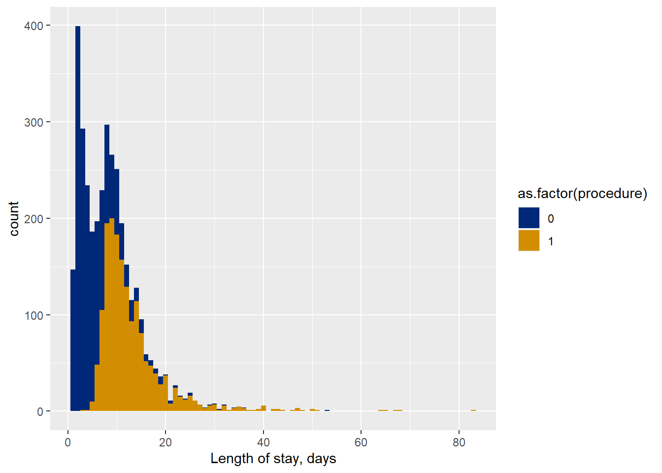
To keep things simple, we’ll start by regressing length of stay only on the procedure and admit variables. Together, they provide k=4 groups of predictor variables.
This asks whether the length of stay differs due to both the procedure type and admit condition.
modpa <- glm(los~procedure+admit, family=poisson, data=azpro)
summary(modpa)
##
## Call:
## glm(formula = los ~ procedure + admit, family = poisson, data = azpro)
##
## Deviance Residuals:
## Min 1Q Median 3Q Max
## -3.3427 -1.1413 -0.4825 0.5084 12.2296
##
## Coefficients:
## Estimate Std. Error z value Pr(>|z|)
## (Intercept) 1.40475 0.01334 105.31 <2e-16 ***
## procedure 0.94910 0.01215 78.08 <2e-16 ***
## admit 0.34265 0.01207 28.38 <2e-16 ***
## ---
## Signif. codes: 0 '***' 0.001 '**' 0.01 '*' 0.05 '.' 0.1 ' ' 1
##
## (Dispersion parameter for poisson family taken to be 1)
##
## Null deviance: 16265.0 on 3588 degrees of freedom
## Residual deviance: 9089.2 on 3586 degrees of freedom
## AIC: 22601
##
## Number of Fisher Scoring iterations: 547.4 Output interpretation
Ideally, the deviance residuals would be symmetrically distributed, as log normal. That’s not the case here. This could be a sign that the Poisson model is not a good one for this data. Perhaps due to over-dispersion.
The values for the coefficient estimates are log counts. The log count for the effect of procedure is 0.949, when exponentiated it is equivalent to about 2.5 days.
Each coefficient has an Wald test to determine if the coefficient value differs from zero. They do.
The interpretation is that a one unit change in procedure adds log count 0.949 days to the length of stay. Since PCTA is keyed as 0 and CABG as 1, this means that the CABG procedure extends the length of stay about 2.5 days compared to PCTA.
The admit status also matters. This variable was keyed at 0 = elective and 1 = urgent. The log count for admit is 0.342, or about 1.4 days. Thus, and urgent admit extends the length of stay about 1.4 days relative to an elective admit.
Whether the intercept differs from zero is usually not interesting. This coefficient represents the log count of days that are not explained by the model. The intercept inflates as the predictor variables are removed, as shown below.
modp <- glm(los~procedure, family=poisson, data=azpro)
summary(modp)
##
## Call:
## glm(formula = los ~ procedure, family = poisson, data = azpro)
##
## Deviance Residuals:
## Min 1Q Median 3Q Max
## -3.3517 -1.4993 -0.5318 0.5354 12.9430
##
## Coefficients:
## Estimate Std. Error z value Pr(>|z|)
## (Intercept) 1.64093 0.01007 163.03 <2e-16 ***
## procedure 0.92563 0.01213 76.31 <2e-16 ***
## ---
## Signif. codes: 0 '***' 0.001 '**' 0.01 '*' 0.05 '.' 0.1 ' ' 1
##
## (Dispersion parameter for poisson family taken to be 1)
##
## Null deviance: 16265.0 on 3588 degrees of freedom
## Residual deviance: 9925.1 on 3587 degrees of freedom
## AIC: 23435
##
## Number of Fisher Scoring iterations: 5And the intercept is reduced further as more variables are factored into the regression.
summary(glm(los~ procedure + admit + sex + age75 + hospital, family=poisson, data=azpro))##
## Call:
## glm(formula = los ~ procedure + admit + sex + age75 + hospital,
## family = poisson, data = azpro)
##
## Deviance Residuals:
## Min 1Q Median 3Q Max
## -3.1981 -1.2081 -0.4208 0.4802 12.6572
##
## Coefficients:
## Estimate Std. Error z value Pr(>|z|)
## (Intercept) 1.4566687 0.0212952 68.404 <2e-16 ***
## procedure 0.9602916 0.0122175 78.600 <2e-16 ***
## admit 0.3266013 0.0121244 26.937 <2e-16 ***
## sex -0.1239367 0.0118125 -10.492 <2e-16 ***
## age75 0.1222160 0.0124491 9.817 <2e-16 ***
## hospital -0.0001489 0.0030984 -0.048 0.962
## ---
## Signif. codes: 0 '***' 0.001 '**' 0.01 '*' 0.05 '.' 0.1 ' ' 1
##
## (Dispersion parameter for poisson family taken to be 1)
##
## Null deviance: 16265.0 on 3588 degrees of freedom
## Residual deviance: 8874.1 on 3583 degrees of freedom
## AIC: 22392
##
## Number of Fisher Scoring iterations: 5Of all the variables, only the hospital is inconsequential. Furthermore, hospital length of stay is reduced 0.124 log counts for males relative to females. All other factors increase the length of stay.
Finally we can test whether one nested model is a better fit than another. The result below indicates that the addition of the admit factor improves the model fit compared to its absence.
anova(modp, modpa, test="Chisq")## Analysis of Deviance Table
##
## Model 1: los ~ procedure
## Model 2: los ~ procedure + admit
## Resid. Df Resid. Dev Df Deviance Pr(>Chi)
## 1 3587 9925.1
## 2 3586 9089.2 1 835.86 < 2.2e-16 ***
## ---
## Signif. codes: 0 '***' 0.001 '**' 0.01 '*' 0.05 '.' 0.1 ' ' 1However, the result below illustrates the addition of a factor to the model that does not improve the fit.
modfull <- glm(los~ procedure + admit + sex + age75 + hospital, family=poisson,  data=azpro)
modless1<- glm(los~ procedure + admit + sex + age75, family=poisson, data=azpro)anova(modless1, modfull, test="Chisq")## Analysis of Deviance Table
##
## Model 1: los ~ procedure + admit + sex + age75
## Model 2: los ~ procedure + admit + sex + age75 + hospital
## Resid. Df Resid. Dev Df Deviance Pr(>Chi)
## 1 3584 8874.1
## 2 3583 8874.1 1 0.0023087 0.9617