Chapter 48 Survival Analysis
library(tidyverse)
library(lubridate)
library(survival)
library(survminer)
library(knitr)
library(kableExtra)
library(coin)
Survival analysis derives its name from experiments designed to study factors that influence the time until discrete death events occur, such as deaths due to cancer or heart disease. When survival is plotted as a function of time, the resulting lines drawn between the data points are called survival curves. The slopes of these curves are called the hazard. The hazard is the rate of death during some period within that curve. For example, if 80% of mice implanted with a tumor die within 1 month the tumor’s hazard is 80% per month.
These ghoulish terms persist even though survival analysis is very useful more generally for studies that involve tracking time to any kind of event, deadly or not.
The two common statistical techniques associated with survival analysis that we will cover are Kaplan-Meier (KM) estimation (including the log rank test to compare two curves) and Cox proportional hazards regression.
KM estimation mostly offers a descriptive way to quantify time to event and survival. KM plots have the characteristic stair step survival curves, where the abscissa is time and the ordinate is survival probability. A KM estimate is the value on these y-axes at a given time. A KM estimate represents the probability of surviving beyond a specific unit of time. For example, when the analysis declares a median survival time for a cancer of 23 months, that implies half of the subjects can be expected to survive beyond 23 months.
KM analysis also allows for testing hypotheses about whether two treatments cause any difference in survival times. The log rank tests employed for this, in effect, test whether the distributions of two survival curves differ from each other. Although these tests report out median survival parameters, they are calculated on the basis of all of the data within a survival curve and are non-parametric.
Cox proportional hazards regression offers a related inferential procedure. The name has three origins. It was invented by Sir David Cox. It is a method to calculate and compare hazard coefficients. It is based upon the assumption that the hazard rates of the two curves being compared are proportional and constant through their full extent. When this latter condition is true, two survival curves can be compared in terms of relative risk.
Cox proportional hazards regression is the basis for making assertions such as, “A person with that cancer has a 20% risk of dying per year.” That statement comes from a survival curve with a hazard rate of 0.2 per year. There may be some study that reports a new treatment, which reduces the hazard rate for that cancer by 50%. The treated hazard rate is now 0.10 per year. Therefore, the treatment reduces the risk of death by half.
48.1 Data records
For a moment I want to distinguish a data frame from a data record. The might be something the researcher keeps while the survival experiment is on-going.
A data frame for a typical survival analysis study is comprised of many cases. Each case represents an independent replicate. The minimal number of variables recorded for each case are as follows:
- The event status
- The duration in time until the event occurred
- A grouping variable (when testing hypotheses)
That dataframe will be minimally necessary to run survival analysis and statistical functions.
In practice, cases come and go throughout an enrollment and follow up period. Our pre-processed records have an ID for the case, an enrollment date or time, a date or time when the event status changed, the event status and the grouping variable, and perhaps some notes.
id <- c(LETTERS[1:4])
start_date <- c("2020-01-14", "2020-01-12", "2020-01-30", "2020-01-29")
end_date <- c("2020-03-29", "2020-01-19", "2020-04-04", "")
status <- c(1,1,0, "")
treatment <- c("placebo","placebo","placebo","placebo" )
notes <- c("", "", "left area, unenrolled", "" )
study <- data.frame(id, start_date, end_date, status, treatment, notes)
kable(study) %>% kable_styling(bootstrap_options = "striped", full_width = F)| id | start_date | end_date | status | treatment | notes |
|---|---|---|---|---|---|
| A | 2020-01-14 | 2020-03-29 | 1 | placebo | |
| B | 2020-01-12 | 2020-01-19 | 1 | placebo | |
| C | 2020-01-30 | 2020-04-04 | 0 | placebo | left area, unenrolled |
| D | 2020-01-29 | placebo |
The event status and end date are intimately linked. An event status is typically entered as a discrete variable code for what occurred on the end date. For example, a status of \(1\) would indicate the event (eg, death) occurred for that case. An event status of \(0\) would indicate the case was censored after that amount of time. The concept of censor is discussed below.
A grouping variable would be something like a treatment variable. For example, a variable named treatment might have two levels, placebo and drug. There may be additional grouping variables.
Given a record of start and end dates/times, we’ll either have to first calculate their difference before passing such data into survival functions, or argue a function so that it will do this given this information.
48.1.1 Deriving times from recorded dates
The duration to an event is something that is calculated during data processing. It is important to pass into the Surv function (below) values in units of time. They should not be simple numeric values.
Survival analysis can be conducted over any time scale.
Scales of days, weeks, months and even years are common. In such designs calendar date variables are commonly used. For example, in a cancer trial a date is recorded for the date a mouse is implanted with a tumor. Subsequently, the date an event (eg, death or censure) occurs is also recorded. The time between these days is then calculated during data processing.
It turns out that dates can be a tricky variable in any computer language due to their imprecision. Shifts such as time zones, the number of days in a month, daylight savings, leap years and even leap seconds occur. Strictly, unlike for seconds (which always have a fixed duration) time variables in units of minutes, hours, days, weeks, months and years (and more) might be approximate unless we account for these shifts. See ?POSIXct for more information.
The lubridate package has several utilities to deal with date/time data. Our main concern is converting date or date/time entries into time values on whatever scale useful for our survival analysis algorithms.
Let’s image the simple case where we record the start dates for enrollment for each case in a study, and then record the date of the event or censure entry.
Note how each vector is that of character strings
start_date <- c("2020-01-14", "2020-01-12", "2020-01-30", "2020-01-29")
end_date <- c("2020-07-29", "2021-01-19", "2020-08-04", "2020-02-29")
The simplest way to calculate the time interval is to first convert the character strings into date objects using the ymd function. Then subtract.
Note how in this case, by default, time units of days are the output. Note this produces a difftime object.
days <- ymd(end_date) - ymd(start_date)
days
## Time differences in days
## [1] 197 373 187 31class(days)## [1] "difftime"When the need is for numeric values as output rather than conversion to difftime, or when calcuating intervals greater than week (difftime does not have units of months or years), the method below takes character strings and produces numeric values in the sought for units.
# illustrating how to calculate four different time scales
# usually there is only one scale of interest
# The divisor can be set to any length: days(7) == week(1)
dateSet <- tibble(start_date, end_date) %>%
  mutate(days = interval(start_date, end_date)/days(1),
         weeks = interval(start_date, end_date)/weeks(1),
         months = interval(start_date, end_date)/months(1),
         years = interval(start_date, end_date)/years(1)
         )
dateSet
## # A tibble: 4 x 6
## start_date end_date days weeks months years
## <chr> <chr> <dbl> <dbl> <dbl> <dbl>
## 1 2020-01-14 2020-07-29 197 28.1 6.48 0.538
## 2 2020-01-12 2021-01-19 373 53.3 12.2 1.02
## 3 2020-01-30 2020-08-04 187 26.7 6.16 0.511
## 4 2020-01-29 2020-02-29 31 4.43 1 0.084748.1.2 Censor
The concept of censor is important in survival studies. Censoring occurs in either of two ways:
- The study period ends without an event having occurred for that case.
- The case is de-enrolled prematurely from an active study for reasons other than meeting the event criterion.
For example, imagine a survival study in mice implanted with experimental tumors where death is the study event. One day, a live mouse jumps out of a cage and escapes from our care, never to be seen again. That mouse should be censored on the date it was lost. A score of \(0\) is entered for the event variable and the date the case was lost is also recorded. It’s gone. Since we don’t know if it died or when it died we have no choice but to record its event as censored.
Censored cases should not be counted as events nor should they be ignored completely once enrolled in a trial. In either circumstance they would skew results if not censored. Censoring reduces the number of subjects at risk that remain in the study, which influences the survival probability calculation (see below).
If a study is designed to last for a limited period, or a decision is made to end the study, then all remaining survivors are censored on that end date.
48.2 Kaplan-Meier estimator
Everyone will recognize the familiar step-down Kaplan-Meier “survival” curve, even though we might not know its name or function. These plot an updated survival probability each time the number at risk (\(N_t\)) in the study changes. The number at risk can change either due to an event (\(D_t\)) or due to censoring (\(C_t\)). \(S_{t+1}\) is the surival probability we are computing due to an event or censoring, while \(S_t\) is the survival probility just before this. \[S_{t+1}=S_t \frac{N_{t+1}-D_{t+1}}{N_{t+1}}\]
Perhaps this is easier to understand through illustration. We begin a study with 10 subjects. We have only one group (no comparisons are involved) and everyone is enrolled simultaneously, to keep it simple. Thus, 10 subjects are at risk of not surviving the protocol. At the intial time, 100% are survivors.
months <- c(0,5,10, 15, 20, 25)
Nt <- c(10,10,8, 7, 6, 5)
Dt <- c("", 1, 1, 1, "", 2)
Ct <- c("", 1, "", "", 1, "")
Stplus1<- c(1, 0.9, 0.788, .675, .675, .404)
kable(data.frame(months, Nt, Dt, Ct, Stplus1))| months | Nt | Dt | Ct | Stplus1 |
|---|---|---|---|---|
| 0 | 10 | 1.000 | ||
| 5 | 10 | 1 | 1 | 0.900 |
| 10 | 8 | 1 | 0.788 | |
| 15 | 7 | 1 | 0.675 | |
| 20 | 6 | 1 | 0.675 | |
| 25 | 5 | 2 | 0.404 |
Exactly five months later one subject dies while a second subject is censored. At the time of these two events there were still 10 subjects at risk. Only the previous survival probability (1), the number of deaths at 5 months (1) and the numbers at risk (10) before this event happened factor into how the survival probability is changed. \(S_{t+1}=(1)\frac{10-1}{10}=0.9\).
The study protocol continues with 8 subjects at risk.
Another five months later a second death occurs, meaning we have to update the survival probability. The number at risk is now 8, since there were previously 1 death and 1 censor. At 10 months, the updated survival probability is \(S_{t+1}=(0.9)\frac{8-1}{8}=0.788\).
The study protocol continues with 7 subjects at risk, awaiting the next event.
Fifteen months after starting the third death occurs. The number at risk prior to this death is 7, due to the loss at the 8 month time point. \(S_{t+1}=(0.788)\frac{7-1}{7}=0.675\).
There are now 6 subjects at risk moving forward.
Twenty months after starting a subject is censored. Nobody dies. The number at risk at this time point was 6 due to the previous death. Since there has been no death, the survival probability remains unchanged. \(S_{t+1}=(0.675)\frac{6-0}{6}=0.675\)
But moving forward there are now 5 subjects at risk in the protocol.
Twenty-five months after starting two subjects die. To update the survival probability the number at risk is down to 5 due to the 1 censor at the prior time. \(S_{t+1}=(0.675)\frac{5-2}{5}=0.404\)
Moving forward 3 subjects are at risk. Their survival probability is 0.404.
The R survival functions will accurately calculate these survival probabilities. Hopefully it is apparent from this example that each updated survival probability is forward looking and applies to the remaining subjects at risk. Furthermore, hopefully it is evident the effect of censoring is to reduce the numbers at risk without affecting survival probability.
More generally, \(S_{t}\) serves as an estimator of the survival function, which predicts the probability of surviving longer than time t.
Median survival times are a very common use of the KM estimator as a descriptive statistic for assessing the influence of some condition on time-to-event. In this paradigm median survival is when \(S_{t}\) is 0.5. Median survival times can be devined from the intercept of the survival curve and a horizontal line extending from \(S_{t}\) = 0.5 on ordinate. The time point corresponding to that intercept is the median survival time.
48.3 Glioma data
Let’s look at some data for exploring statistical inference.
The glioma data set below comes from the coin package. Note it contains 37 cases listing the survival times for people with either Grade3 or GBM gliomas. Notice also that it contains a few grouping factors, including histology, sex, and group.
We’ll just focus on survival associated with histology, which you’ll recognize as two different types of glioma.
The first step is to create a survival model of the data. The Surv function from the survival package in conjunction with the survfit function summarizes the events while calculating the survival probability for each event and its associated time points (which are in months), along with some useful summary statistics.
Hopefully the formula Surv(time, event) ~ 1 below strikes as reminiscent of that which is used in regression. Here, the survfit function calculates the numbers at risk, the numbers of events and the survival, along with standard error and confidence interval for each time point. This is how to regress the data WITHOUT accounting for the effects of any of the predictors. This is being done to illustrate a couple of points.
modelAll <- survfit(Surv(time, event) ~ 1, data = glioma)
summary(modelAll)
## Call: survfit(formula = Surv(time, event) ~ 1, data = glioma)
##
## time n.risk n.event survival std.err lower 95% CI upper 95% CI
## 5 37 1 0.973 0.0267 0.922 1.000
## 6 36 1 0.946 0.0372 0.876 1.000
## 8 35 4 0.838 0.0606 0.727 0.965
## 9 31 1 0.811 0.0644 0.694 0.947
## 11 30 1 0.784 0.0677 0.662 0.928
## 12 29 1 0.757 0.0705 0.630 0.908
## 13 28 1 0.730 0.0730 0.600 0.888
## 14 27 3 0.649 0.0785 0.512 0.822
## 15 24 1 0.622 0.0797 0.483 0.799
## 19 23 1 0.595 0.0807 0.456 0.776
## 20 22 1 0.568 0.0814 0.428 0.752
## 25 21 2 0.514 0.0822 0.375 0.703
## 31 18 1 0.485 0.0824 0.348 0.677
## 32 17 1 0.456 0.0824 0.321 0.650
## 34 16 1 0.428 0.0820 0.294 0.623
## 36 15 1 0.399 0.0813 0.268 0.595
## 53 8 1 0.349 0.0851 0.217 0.563modelAll## Call: survfit(formula = Surv(time, event) ~ 1, data = glioma)
##
## n events median 0.95LCL 0.95UCL
## 37 23 31 15 NAThe overall median survival calculated for these 37 cases is 31 months (95% CI is 15 to NA).
modelAll## Call: survfit(formula = Surv(time, event) ~ 1, data = glioma)
##
## n events median 0.95LCL 0.95UCL
## 37 23 31 15 NANow let’s focus on comparing the two groups under the histology variable to ask whether the type of tumor influences survival. We are NOT going to factor in the effects of age, sex or the group variable, in order to keep things simple.
First we change the formula from above:
modelHis <- survfit(Surv(time, event) ~ histology, data = glioma)
summary(modelHis)
## Call: survfit(formula = Surv(time, event) ~ histology, data = glioma)
##
## histology=GBM
## time n.risk n.event survival std.err lower 95% CI upper 95% CI
## 5 20 1 0.95 0.0487 0.8591 1.000
## 6 19 1 0.90 0.0671 0.7777 1.000
## 8 18 4 0.70 0.1025 0.5254 0.933
## 11 14 1 0.65 0.1067 0.4712 0.897
## 12 13 1 0.60 0.1095 0.4195 0.858
## 13 12 1 0.55 0.1112 0.3700 0.818
## 14 11 3 0.40 0.1095 0.2339 0.684
## 15 8 1 0.35 0.1067 0.1926 0.636
## 20 7 1 0.30 0.1025 0.1536 0.586
## 25 6 1 0.25 0.0968 0.1170 0.534
## 31 5 1 0.20 0.0894 0.0832 0.481
## 36 4 1 0.15 0.0798 0.0528 0.426
##
## histology=Grade3
## time n.risk n.event survival std.err lower 95% CI upper 95% CI
## 9 17 1 0.941 0.0571 0.836 1.000
## 19 16 1 0.882 0.0781 0.742 1.000
## 25 15 1 0.824 0.0925 0.661 1.000
## 32 13 1 0.760 0.1048 0.580 0.996
## 34 12 1 0.697 0.1136 0.506 0.959
## 53 7 1 0.597 0.1341 0.385 0.927The two groups differ in median survival. For the cases with GBM it is 14 months (95%CI is 11 to 31 months). The median survival for Grade3 cases is undefined. That’s because the survival rate is greater than 0.5…they have not reached the median point!
modelHis## Call: survfit(formula = Surv(time, event) ~ histology, data = glioma)
##
## n events median 0.95LCL 0.95UCL
## histology=GBM 20 17 14 11 31
## histology=Grade3 17 6 NA 53 NA48.4 Kaplan-Meier plots
The survival package has base plotting functions, but we use functions in the survminer package to generate ggplots of survival curves.
First a bare bones plot of the unsegmented data. Notice how the median surival line is drawn. Also notice the discrete nature of the 95% confidence intervals (shaded).
ggsurvplot(modelAll,
           surv.median.line = "hv", # Specify median survival
           palette = c("#002878"))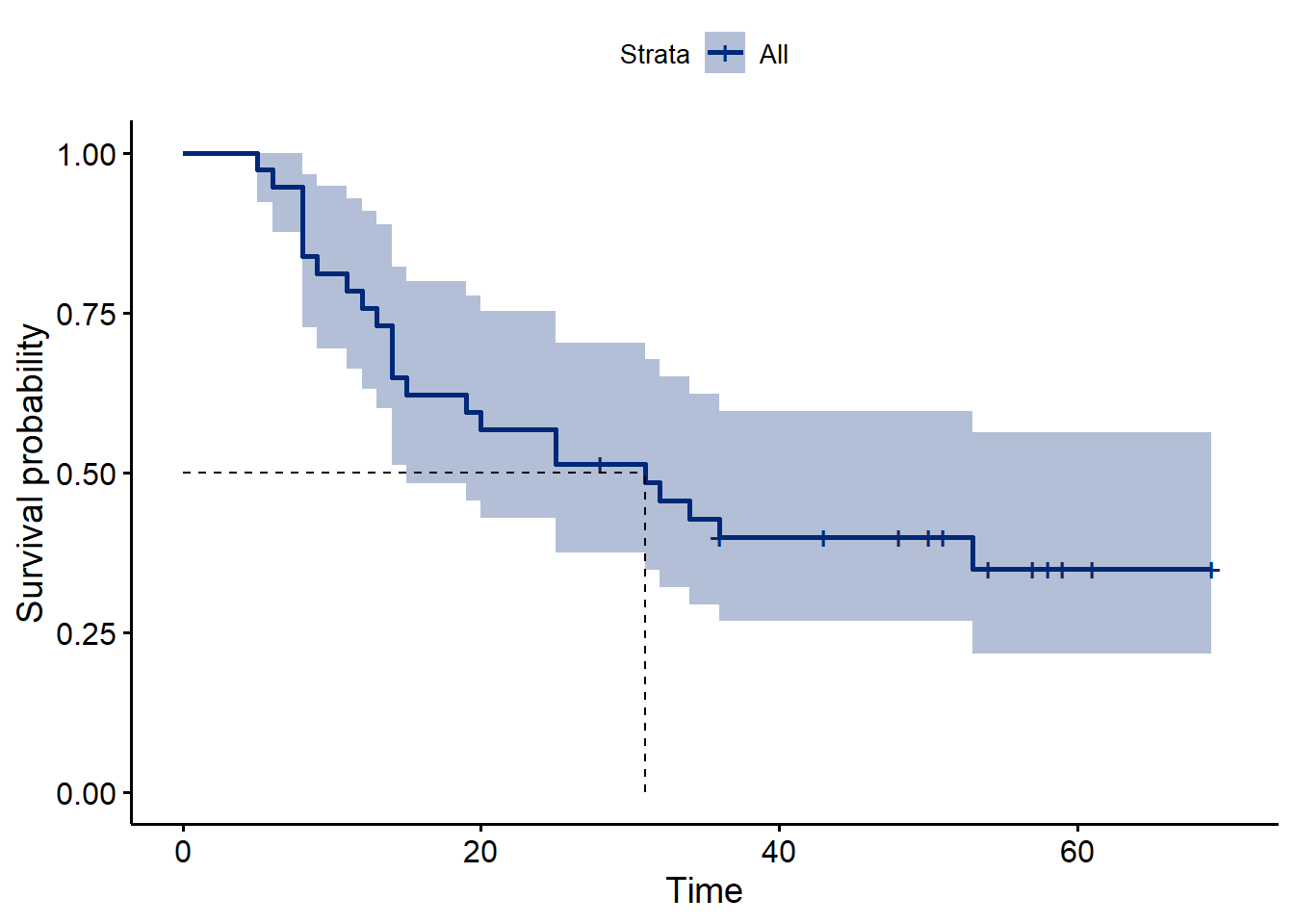
Figure 48.1: Overall survival in the glioma data, irrespective of tumor type.
Next we plot the survival curves based upon the histology variable. Note how Grade3 survival never reaches 0.5, thus a median survival time is not possible to calculate.
ggsurvplot(modelHis,
          conf.int = TRUE,
          surv.median.line = "hv", # Specify median survival
          ggtheme = theme_bw(), # Change ggplot2 theme
          palette = c("#002878", "#d28e00"))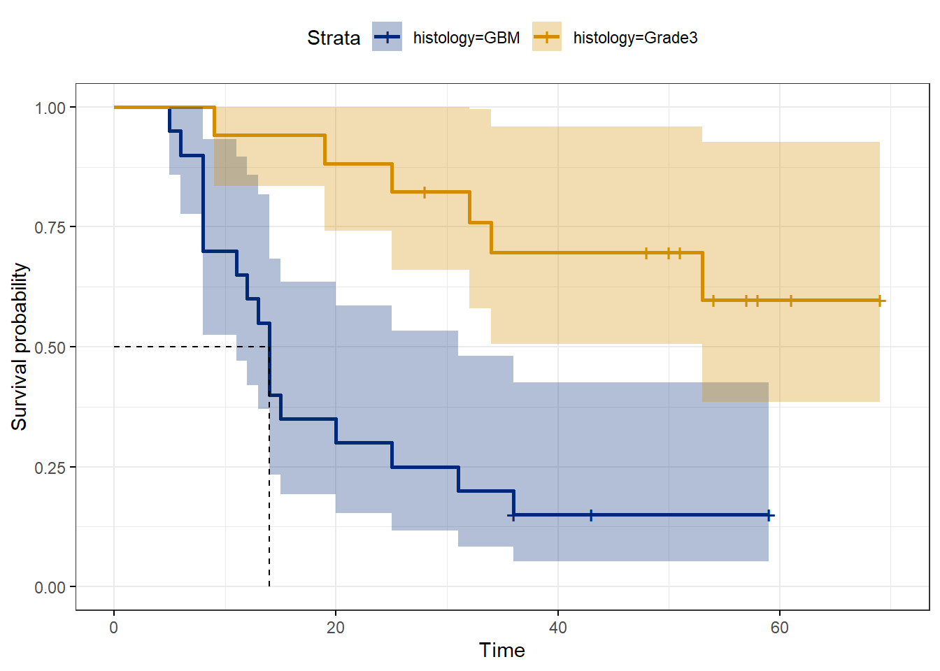
Figure 48.2: Glioma survival by type of tumor.
48.5 Log rank tests
The key question we address with log rank testing is whether survival differs between GBM and Grade3.
It is a very simple question. If true, it implies the two conditions differ. The experimental researcher is typically only interested in survival curve differences and uninterested in hazard ratios or relative risk. For example, in an implanted tumor model, the researcher wishes to manipulate the immune system in some way to test if it alters survival. Period.
Log rank tests (there are several) are nonparametric tests for comparing survival distributions and thus answering this question.
The differences between the various log rank tests is beyond the intended scope. See coin::?logrank_test for an entry into the broader universe of the various tests, their features and arguments and use cases.
In the case of the glioma data, we test the null hypothesis that the survival distributions for GBM and Grade3 are equivalent.
\(H_0\): The GBM and Grade3 survival distributions are the same. \(H_1\): The GBM and Grade3 survival distributions differ.
The parameterless wishy-washiness of the null hypothesis should remind us of nonparametric hypothesis tests. There is no parameter here. The log rank test is a nonparametric test, which only evaluate the relative locations of the two distributions without consideration of their central tendency or any other parameter.
It is very common to summarize the differences between survival curves through describing their relative median survival times. Therefore, median survival times serve as a useful pseudo-parameter. However, the log rank test is definitely not comparing medians.
One can imagine instances where the values of median are roughly the same (if not identical) yet the distributions differ markedly, because survivals diverge at times beyond a common median survival time point. The log rank tests are likely to pick up those differences in survival, because they factor into their calculations the full breadth of the survival curves.
The default mode for the survdiff function in the survival package runs a Mantel-Haenszel log rank test producing a \(\chi^2\) test statistic with 1 degree of freedom. \[\chi^2=\frac{(\sum O_{1t}-\sum E_{1t})^2}{\sum Var(E_{1t})}\]
Here \(\sum O_{it}\) and \(\sum E_{it}\) are the sum of the observed and expected number of events in group 1 over all event times. The denominator is the sum of the variances for all events, \[Var(E_{1t})=\frac{N_{1t}\times N_{2t}\times (N_t-O_t)}{N_t^2\times(N_t-1)}\] Here \(N\) represents the total numbers at risk at a given time point, while \(N_1\) and \(N_2\) are the at risk within each group.
Here is how to run the test.
survdiff(Surv(time, event) ~ histology, data = glioma)## Call:
## survdiff(formula = Surv(time, event) ~ histology, data = glioma)
##
## N Observed Expected (O-E)^2/E (O-E)^2/V
## histology=GBM 20 17 8.82 7.57 13.4
## histology=Grade3 17 6 14.18 4.71 13.4
##
## Chisq= 13.4 on 1 degrees of freedom, p= 2e-04Note that the column labeled (O-E)^2/E reports the \(\chi^2\) values for each of the two groups. When summed, they become the classic Mantel-Cox log rank test statistic, which can be used as an alternative for inference rather than the default.
The column sum is \(\chi^2=12.28\) with 1 degree of freedom. Use the chisq distribution to compute its p-value:
pchisq(12.28, df=1, lower.tail=F)## [1] 0.0004578384Although the test statistic and p-values for these two log rank tests are similar, they are not identical. The values should agree in well-powered experiments. To avoid p-hacking temptations, make the decision in advance to use one or the other.
Nevertheless, either test generates an extreme \(\chi^2\) test statistic and corresponding low p-value, below the typical type1 error threshold of 0.05. On this basis reject the null hypothesis that the survival associated with both cancers is the same.
48.5.1 Write up of log rank test
Survival with Grade3 (median survival = undetermined months, 95%CI = 53 to undetermined) differs from survival with GBM (median survival = 14 months, 95%CI = 11 to 31 months; Mantel-Haenszel log rank test, chisq= 13.4, p=2e-4).
48.5.2 Comparing more than two survival curves
The log rank test can be performed on multiple curves simultaneously. There are two inferential options.
- Conclude from the overall chi-square test that at least one of the treatment levels differs from the others, using the bloody obvious test to draw further conclusions.
- Use the overall chi-square test as an omnibus test, much like an ANOVA F-test, granting permission to perform multiple post-hoc comparisons.
For the latter we run the pairwise_survdiff function from the survminer package. This is very simple to execute. Selecting “none” as a p-value adjustment method allows for pulling out a vector of unadjusted p-values, to focus on only the comparisons of interest.
48.6 Cox proportional hazards analysis
Log rank testing only leaves us with a test statistic.
Cox proportional hazards analysis is invoked when the researcher seeks to describe the treatment effect by deriving a quantitative parameter from the survival data. Specifically, for when one wants to describe quantitatively how survival rates are influenced by treatment conditions.
The Cox model is otherwise known as the hazard function.
The jargon used to define the survival rate of a treatment condition is the hazard, \(\lambda(t)\). The baseline hazard, \(\lambda_0(t)\), is the survival rate in the control setting, in the absence of any treatment condition. The Cox model defines the hazard as a function of a linear combination of predictor variables, \(X\): \[\lambda(t) = \lambda_0(t)\times e^{\beta_1 X_1+\beta_2 X_2..+beta_p X_p}\] In the simple case where the predictor variable \(X\) is discrete at two levels, such as a control or a treatment, for the control \(X=0\) then \[\lambda(t) = \lambda_0(t)\], or is the baseline hazard.
When treatment is present, \(X=1\) then \[\lambda(t) = \lambda_0(t)\times e^{\beta X}\] or \[\frac{\lambda(t)}{\lambda_0(t)}=e^{\beta}\] Finally, natural log transformation creates a linear form of the equation \[log(\frac{\lambda(t)}{\lambda_0(t)})=\beta\]
- \(e^{\beta}\) equals the hazard ratio or the relative risk
- \(\beta\) equals the log hazard ratio or log relative risk
This (and a bit more mathematical proofing of the Cox model) implies that the ratio of the two hazards are a constant and independent of time, from whence the term ‘proportional’ is derived. In other words, the procedure is based upon the assumption that the hazard ratio is constant across all times of the study period.
48.6.1 Cox proportional hazards regression of glioma
In the code below Cox regression is executed on the glioma data, testing only the histology variable for the difference in survival between the GBM and Grade3 gliomas. Again, we ignore the other predictors.
modelHis.cox <- coxph(Surv(time, event) ~ histology, data = glioma)
modelHis.cox
## Call:
## coxph(formula = Surv(time, event) ~ histology, data = glioma)
##
## coef exp(coef) se(coef) z p
## histologyGrade3 -1.6401 0.1940 0.4881 -3.36 0.000779
##
## Likelihood ratio test=13.24 on 1 df, p=0.0002738
## n= 37, number of events= 23print("/////////////////////////////////////")## [1] "/////////////////////////////////////"print("/////////////////////////////////////")## [1] "/////////////////////////////////////"summary(modelHis.cox)## Call:
## coxph(formula = Surv(time, event) ~ histology, data = glioma)
##
## n= 37, number of events= 23
##
## coef exp(coef) se(coef) z Pr(>|z|)
## histologyGrade3 -1.6401 0.1940 0.4881 -3.36 0.000779 ***
## ---
## Signif. codes: 0 '***' 0.001 '**' 0.01 '*' 0.05 '.' 0.1 ' ' 1
##
## exp(coef) exp(-coef) lower .95 upper .95
## histologyGrade3 0.194 5.156 0.07452 0.5049
##
## Concordance= 0.709 (se = 0.041 )
## Likelihood ratio test= 13.24 on 1 df, p=3e-04
## Wald test = 11.29 on 1 df, p=8e-04
## Score (logrank) test = 13.6 on 1 df, p=2e-0448.6.2 Interpretation of Cox regression output
From the output above, printing the regression model alone is comprehensive except for confidence intervals. Passing the model into the summary function pulls out this and some additional detail
48.6.2.1 Log hazard ratio/relative risk
The coef value corresponds to \(\beta\) from the hazard equation above, which in general terms equals \(log(\frac{\lambda(t)}{\lambda_0(t)})\). Thus we can say the log hazard ratio is -1.6401.
But what does that actually mean, and who is what in this case?
First, recall R’s quirk in regression. R does not know if we want GBM or Grade3 to be the intercept. When we don’t tell it, that means that it will go choose the first alphanumerical as the intercept. In this case, that is GBM.
Remember that \(\lambda\) symbolizes survival rates. And there are two survival rates of interest in this case: one for GBM and another for Grade3. Furthermore, we can bloody obvious tell from the plot above that the survival rate for Grade3 is larger than that for GBM. Think about that carefully for a moment before reading on.
Log fractions can confuse. Here we know that \(log(\lambda(t))-log(\lambda_0(t))=-1.6401\). The negative value of this difference means that \(\lambda_0(t)\) must be greater than than \(\lambda(t)\). Therefore we can deduce that this R function has coerced Grade3 as the denominator, or \[coef=log \ hazard \ ratio=log(\frac{\lambda_{GBM}(t)}{\lambda _{Grade3}(t)})=-1.6401\]
The z statistic and p-value for coef correspond to a Wald test (a ratio of the coefficient value to its SE). This tests the null hypothesis that coef= 0 (if two survival rates are the same, their ratio is 1, null coef=log(1)=0). If the null is true it would indicate there is no evidence that factor associated with that coefficient affects the log hazard ratio.
48.6.2.2 Hazard ratio/relative risk
Now for the exp(coef). This is the hazard ratio, otherwise known as the relative risk. Either of these two terms are used commonly and interchangeably. They also have greater descriptive efficacy than the log hazard ratio simply because logs tend to confuse people.
Hazard == survival rate. It is worth repeating that the hazard ratio nothing more complicated than a ratio of survival rates….and no logs are involved. \[\frac{\lambda(t)}{\lambda_0(t)}=e^{\beta}=\frac{\lambda_{GBM}(t)}{\lambda _{Grade3}(t)}=0.1940\]
Since the value of the hazard ratio is below 1, and \(\lambda\) symbolizes survival rates, this result shows that the survival rate with GBM is lower than the survival with Grade3 tumors. That is bloody obvious from inspection of the plot above.
In fact, the GBM survival rate is 19.4% the survival rate for Grade3. Or we can say the relative risk of death due to Grade3 tumors is 19.4% of GBM tumors. or we can say hazard associated with Grade3 tumors is 19.4% of that for GBM.
Or we would just report the hazard ratio as a descriptive: Grade3 to GBM HR = 0.194.
Now please note the exp(-coef) column. This is merely the reciprocal of the hazard ratio. A personal preference might be to use this. Is so, one would say that the hazard rate of GBM is 5.156 times greater than that for Grade3. Alternately the relative risk of GBM to Grade3 glioma is 5.156.
48.6.2.3 Confidence interval
We can say that there is a 95% chance the hazard ratio (or relative risk) of Grade3 to GBM tumor has the values between 0.07452 and 0.5049.
It takes professional judgement to decide whether that range is scientifically meaningful. Is is reasonable to think Grade3 tumors are anywhere from a tenth to half as deadly as GBM. An expert in the field could assess that conclusion. Importantly the confidence interval does not include the value of 1, which for a ratio would indicate the two tumors have the same hazard.
48.6.2.4 Statistical tests
Finally on to the statistical tests.
This function by default generates 3 inferential tests and the researcher chooses one of these via preference. In well-powered experiments all three should converge to a similar conclusion but won’t have the exact same values. On close calls, when the researcher decides in advance of testing which one to use the temptation to p-hack is averted.
The log rank test is handled in the section above. The Wald test won’t be discussed here in detail. It is an extension of the Wald test used above for the single coefficient value. The main difference is that the Wald test for the overall regression handles many coefficients simultaneously. That’s not an issue in this simple case, but it would be if other predictor variables were added to the regression model.
Likelihood ratio tests are most commonly used. They always compare the fits of two different models, usually nested, to a common data set.
The likelihood function first calculates parameter values for each model that are most likely to fit the data the best. The test statistic is then the ratio of these two likelihoods, generally: \[LR=-2log\frac{L(resricted \ model)}{L(full \ model)}=2(loglike(full \ model)-loglike(restricted \ model)\] LR is distributed approximately \(\chi^2\) with degrees of freedom equal to the number of restricted parameters.
In this case the full model is that which includes the histology variable and corresponding \(\beta\) coefficient as a parameter. The restricted model lacks any predictor variable altogether. The restrictive model is the overall survival of glioma, irrespective of tumore type. Therefore, it helps answer the question: Does the histology variable influence survival at all, relative to the overall survival.
Clearly, the answer is yes.
48.6.3 Write up
We can conclude that survival with GBM is approximately one-fifth that for Grade3 glioma (hazard ratio = 0.194, hazard ratio 95%CI 0.07 to 0.509, Cox proportional hazards regression, LR = 13.24, df=1, p=0.00027, n =37 with 23 events).
Or we could conclude that survival with GBM is approximately one-fifth that for Grade3 glioma (relative risk = 0.194, relative risk 95%CI 0.07 to 0.509, Cox proportional hazards regression, LR = 13.24, df=1, p=0.00027, n =37 with 23 events).
48.7 Summary
- Thinking of survival analysis as time-to-event can broaden the experiments we might apply this design to.
- Log rank tests are a straight forward nonparametric method of asking whether two survival curves differ.
- Cox proportional hazards regression is used to obtain quantified parameters associated with a treatment model.
- We covered a simple binary event scenario, but events can be more complex than this (eg, two or more outcome events other than censor).
This chapter is intended to serve as an introduction to survival analysis for the researcher. The Cox proportional hazards model is flexible and can accommodate considerably more intricate statistical designs then listed here, including multiple variables and interaction tests between them. None of this is covered here.
This is probably one of those areas of statistics where a reliable textbook should be consulted when diving into more sophisticated experiments than shown here. Here’s a good discussion on the different books available and which might best suite you.