Chapter 8 R Learnings for now
library(tidyverse)
library(datapasta)
library(viridis)
Now that we have R and RStudio up and running, and we’re talking about variables, let’s turn our attention to the important things to learn about R this week.
I don’t think it is possible to talk about variables without the ability to visualize them. To visualize data we need to get it into our software. We frequently need to also subset, transform & summarize variables. Then we need to plot…which involves thinking about the structure of plots.
This chapter has most of what you need…code-wise…to work on the homework and inclass assignments for this we. You will also need to know how to plot histograms and distribution functions. See section 17.4.2.2 for the latter.
8.1 The whole R thing
First, let’s cover some R syntax/logic stuff.
If something isn’t working check your spelling, commas and parentheses. Mistakes with these explain at least 90% of errors.
8.1.1 Words matter
R is case sensitive and cannot parse misspellings. Precision matters. This causes 45% of errors.
8.1.2 Functions & arguments
Arguments are placed inside () following the function name. Anything inside () will be an argument. Commas always separate arguments. Data objects can be arguments.
We pass “data” into functions and choose arguments that give us the results we need.
A very common error is to forget a comma or parenthesis. This causes 45% of errors, too.
# x is a variable with 5 values and 1 missing value
# x is a data object
x <- c(1, 2, NA, 3, 4 ,5)
# variables can be arguments in functions
# na.rm = T is also an argument, guess what it does?
# We usually won't get a function result unless R
# is told what to do with missing values
mean(x, na.rm = T)
8.1.3 Functions work inside other functions
Scripting involves building chains of functions.
The pipe function, %>%, from the dplyr package will be your best friend in the course if you allow it. In English, %>% means ‘then’ or ‘next.’
Let’s compare it to old fashioned R syntax.
Conceptually, chaining is a sequential process and oftentimes the sequence matters.
# old fashioned R syntax,
# sometimes hard to read and write, but works NTTAWWT
# actually performs from right to left:
# pretend I'm a data object
me <- "tj murphy"
# here's a script for my workday
work(commute(shower(breakfast(walk_dog(bathroom(wake_up(me)))))))
# here's the same script but with piping
# piping is more natural
me %>%
  wake_up() %>%
  bathroom() %>%
  walk_dog() %>%
  breakfast() %>%
  shower() %>%
  commute() %>%
  work()
# I saw this analogy on twitter and wish I'd invented it
8.1.4 Divide by two
That’s slang for taking big problem, cutting it into parts, and then cutting the parts again, and so on until the parts are digestible enough to be solved.
Nobody writes 100 lines of script at once, then runs it, and it works.
A good scripting process is working in steps.
Make sure each works before chaining it to the next. And if we’re not getting what we want, maybe our steps are not in the right order?
8.1.5 Steal my code
Copy/paste is a great way to start coding. Then custom fit it for the task at hand.
Most of the code in this book was written that way.
8.1.6 Nine MUST KNOW functions for now
read_csv converts a csv file on your machine into a tibble, which is a dataframe.
pcd <- read_csv("datasets/precourse.csv")## Rows: 464 Columns: 6## -- Column specification --------------------------------------------------------
## Delimiter: ","
## chr (1): sex
## dbl (4): term, enthusiasm, height, fav_song##
## i Use `spec()` to retrieve the full column specification for this data.
## i Specify the column types or set `show_col_types = FALSE` to quiet this message.Here is a goal: Generate some descriptive statistics, for only valid heights of male and female biostats students, in units of inches rather than centimeters.
Here is a solution that involves six functions from the dplyr package.
%>%, select, filter, mutate, group_by, summarise
pcd %>%
  select(height, sex) %>%
  filter(height > 125 & height < 250) %>%
  mutate(height = height/2.54) %>%
  group_by(sex) %>%
  summarise(mean = mean(height),
            sd = sd(height),
            n = length(height))
## # A tibble: 2 x 4
## sex mean sd n
## <chr> <dbl> <dbl> <int>
## 1 Female 64.7 2.86 284
## 2 Male 70.2 3.07 168Think about these functions:
%>%aka pipe, chains functions together in a logical orderselectchooses variables (columns) from a dataframefilterchooses rows from a dataframemutateis how we transform variables, clever, huh?group_bysegmentation, based upon values of the argued variablesummarisecalculates any summary statistic you can imagine
The ninth function to know for now is ggplot, which we will cover below.
8.1.7 You have options
There are many ways to do the same thing in R, or pretty much the same thing. The important thing is to make sure we get the right thing.
# need a data frame object of random normal values?
a <- rnorm(5)
b <- rnorm(5)
oneway <- data.frame(a, b)
another <- data.frame(a = rnorm(5), b = rnorm(5))
prettyMuchTheSame <- tibble(a, b)
8.2 Working with variables in R
The sections below are a quick primer on R data entry, inspection, manipulation/summation and visualization with ggplot.
The focus here is conceptual with simple quick examples to help you get started.
They are intended for you to copy/paste and play with.
8.3 Entering data
There are three main ways:
- Type from your lab notes by keyboard into an R source, such as an R script file.
- Copy to clipboard from some file, paste using the
datapastapackage addin. - Read from a file.
8.3.1 Typing in variables and making a data frame
Let’s say we have some data in a lab notebook.
These are results from a small pilot experiment comparing the effect on neurological function of knockout of the ND4 gene to wild-type. Oh, and lab meeting is in 10 minutes.
The knockout and wild-type are two values of the variable genotype, which is sorted.
Neurological function is assessed using the 6-value disability status scale, which is an ordered variable.
Both variables are discrete.
Saving the Rscript (or Rmarkdown) file stores the data.
The function tibble() creates a tidyverse data frame.
# understand the logic of creating vector objects for the
# independent and the dependent variables
# note how a tibble-type data frame is created

# vector objects represent the variables
genotype <- c(rep("wt", 3), rep("ND4", 3))
DSS_score <- as.integer(c(0,1,1,5,3,5))

# put the variables in a data frame object
results <- tibble(genotype, DSS_score); results
## # A tibble: 6 x 2
## genotype DSS_score
## <chr> <int>
## 1 wt 0
## 2 wt 1
## 3 wt 1
## 4 ND4 5
## 5 ND4 3
## 6 ND4 5ggplot(results, aes(x=genotype, y=DSS_score)) +
geom_jitter(height=0, width=0.3, size=4)## Warning in (function (kind = NULL, normal.kind = NULL, sample.kind = NULL) :
## non-uniform 'Rounding' sampler used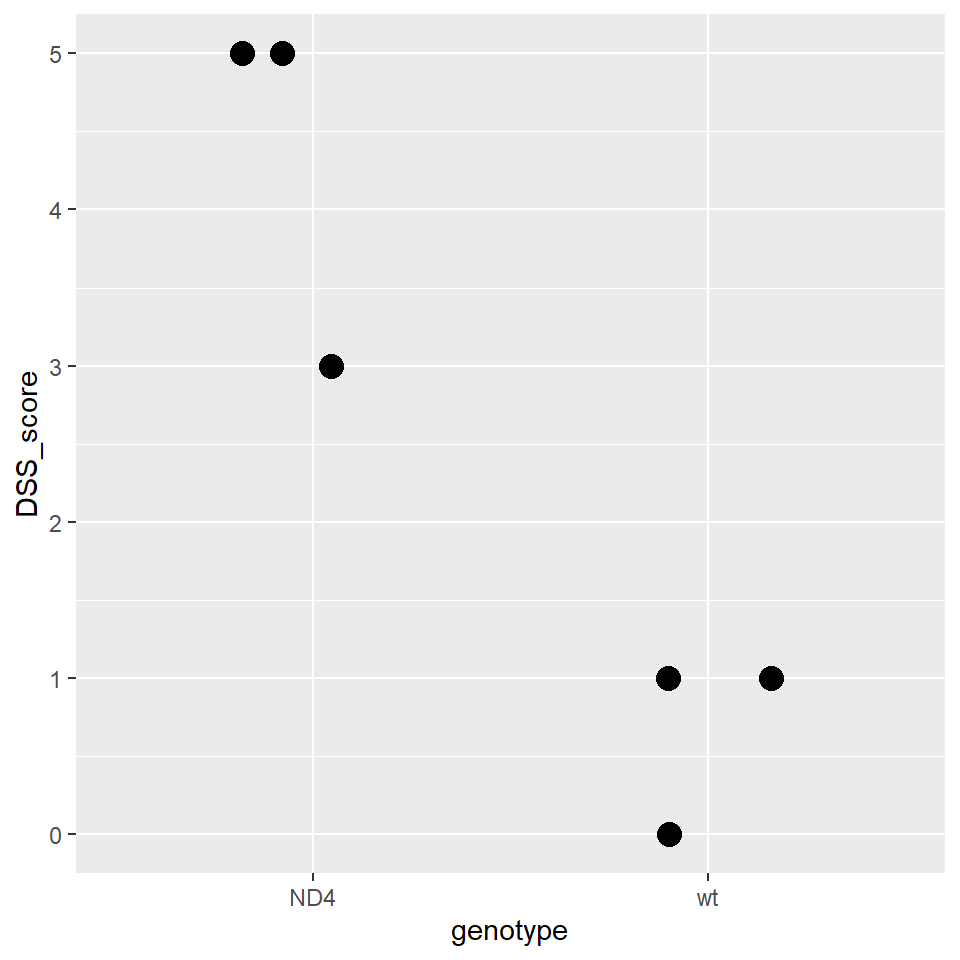
Woot! Ready to present a table and a plot in lab meeting!
8.3.2 Using datapasta
This is a good way to import large chunks of data from other formats.
View a data file on your machine, such as an excel sheet, select the rows and columns of interest.
Copy the data you want to your machine’s clipboard.
In an Rscript or chunk, name an empty object (eg,
song <-c()).Place the cursor inside the parentheses.
Click on the Addins icon below the RStudio menu bar and select an option.
Here I copied the fav_song column (including header) from the precourse.csv file. Probably due to that header, datapasta coerced the values as characters. Some munging will be necessary to clean things and turn everything into numeric values. But at least it’s in R now. Woot.
song <-c("fav_song", NA, NA, NA, NA, NA, NA, NA, NA, NA, NA, NA, NA, NA, NA, NA, NA, NA, NA, NA, NA, NA, NA, NA, NA, NA, NA, NA, NA, NA, NA, NA, NA, NA, NA, NA, NA, NA, NA, NA, NA, NA, NA, NA, NA, NA, NA, NA, NA, NA, NA, NA, NA, "570", "576", "232", "204", "524", "252", "588", "201", "212", "221", NA, "265", "294", "217", "246", "481", "480", "200", "180", "210", "203", "210", "172", "255", "375", "698", "234", "242", "256", "288", "272", "273", "601", "293", "260", "120", "300", "147", "272", "202.2", "274", "293", "262", "555", "362", "260", "180", "237", "300", "373", "121", "361", "179", "169", "201", "194", "246", "139", "210", "234", "292", "217", "412", "172", "289", "214", "180", "448", "180", "207", "74", "253", "256", "243", "187", "420", "200", "235", "185", "246", "172", "258", "213", "188", "258", "201", "214", "210", "230", "5421", "259", "222", "171", "184", "220", "225", "295", "240", "250", "204", "208", "254", "341", "233", "232", "455", "423", "246", "570", "319", "0", "205", "240", "260", "126", "480", "210", "226.93", "0", "300", "180", "298", "290", "202", "194", "246", "232", "210", "150", "236", "174", "260", "300", "565", "273", "245", "360", "174", "276", "293", "460", "240", "583", "90", "180", "240", "244", "127", "210", "211", "240", "220", "241", "180", "230", "180", "198", "133", "272", "293", "296", "230", "212", "195.6", "187", "200", "234", "200", "240", "295", "183", "216", "286", "192", "270", "360", "262", "268", "234", "1560", "197", "261", "279", "195", "251", "295", "461", "360", "218", "185", "250", "257", "210", "199", "210", "210", "200", "261", "237", "226", "331", "261", "190", "222", "180", "284", "120", "255", "222", "3", "200", "235", "277", "314", "249", "75", "300", "277", "250", "241", "209", "250", "200", "210", "402", "360", "205", "345", "252", "305", "201", "170", "213", "656", "240", "339", "172", "263", "239", "135", "210", "230", "185", "292", "210", "432", "200", "192", "21", "215", "240", "240", "200", "480", "247", "200", "253", "230", "355", "214", "332", "2450", "300", "180", "237", "379", "516", "180", "184", "218", "222", "194", "160", "234", "238", "208", "250", "123", "240", "226", "237", "176", "200", "192", "347", "255", "254", "255", "240", "480", "240", "456", "223", "236", "201", "190", "226", "300", "288", "681", "180", "352", "270", "245", "180", "229", "180", "221", "320", "217", "236", "352", "233", "214.8", "262", "179", "221", "227", "241", "180", "2640", "364", "240", "382", "243", "204", "185", "240", "298", "155", "216", "24840", "180", "202")8.3.3 Reading a file
Of the three data entry methods, reading a file is the most reproducible.
Raw data are read from files into R objects using a script. The data object represents all the values from the file and is now in the environment. The object can be worked on to fix, segment, summarize, and visualize the data.
After the initial read step, the raw data file remains untouched. Which is very good. As a general rule, just save the script and never write over raw data because doing so changes the raw data.
When you need to work on the data later in a new R session, just re-run the saved script, including the read step.
This is a very different way of working with data compared to using GUI-based software. We don’t create and save all sorts of new sheets of edited or interpreted data. Or overwrite the original data sheet.
We just write a script, and change it until we get exactly what we want. The script provides the reproducible record of how the data was manipulated.
We’ll (mostly) use .csv files as a data source in this course.
The same basic reading approach used for that is applicable to all kinds of other data sources. Many different R functions exist to read from many different types of data sources.
Here’s how to import the precourse survey data using the read_csv function from the tidyverse readr package.
# my working directory has a subdirectory named datasets
# the precourse.csv file is in the datasets folder
# If the csv file is in your working directory, just do: pcd <- read_csv("precourse.csv)
pcd <- read_csv("datasets/precourse.csv")
## Rows: 464 Columns: 6## -- Column specification --------------------------------------------------------
## Delimiter: ","
## chr (1): sex
## dbl (4): term, enthusiasm, height, fav_song##
## i Use `spec()` to retrieve the full column specification for this data.
## i Specify the column types or set `show_col_types = FALSE` to quiet this message.Inspect the data to make sure it is what you think it is.
# get in the habit of inspecting data, several ways
str(pcd)
## spec_tbl_df [464 x 6] (S3: spec_tbl_df/tbl_df/tbl/data.frame)
## $ term : num [1:464] 2014 2014 2014 2014 2014 ...
## $ enthusiasm: num [1:464] 6 7 7 10 7 5 5 10 7 10 ...
## $ height : num [1:464] 170 158 163 168 168 ...
## $ friends : num [1:464] 685 154 1333 0 250 ...
## $ sex : chr [1:464] "Female" "Female" "Female" "Female" ...
## $ fav_song : num [1:464] NA NA NA NA NA NA NA NA NA NA ...
## - attr(*, "spec")=
## .. cols(
## .. term = col_double(),
## .. enthusiasm = col_double(),
## .. height = col_double(),
## .. friends = col_number(),
## .. sex = col_character(),
## .. fav_song = col_double()
## .. )
## - attr(*, "problems")=<externalptr>head(pcd)## # A tibble: 6 x 6
## term enthusiasm height friends sex fav_song
## <dbl> <dbl> <dbl> <dbl> <chr> <dbl>
## 1 2014 6 170 685 Female NA
## 2 2014 7 158. 154 Female NA
## 3 2014 7 163. 1333 Female NA
## 4 2014 10 168 0 Female NA
## 5 2014 7 168. 250 Female NA
## 6 2014 5 157 476 Female NAview(pcd)There are a handful of functions in R land for reading .csv data. They don’t all work the same,
8.4 Subsetting, transforming and summarizing data
The functions select, filter and group_by are subsetting functions.
The function mutate is a workhorse function to rescale data through transformation.
The function summarise let’s us calculate whatever summary statistic we wish.
pcd %>%
  select(height, sex) %>%
  filter(height > 125 & height < 250) %>%
  mutate(height = height/2.54) %>%
  group_by(sex) %>%
  summarise(mean = mean(height),
            sd = sd(height),
            n = length(height))
## # A tibble: 2 x 4
## sex mean sd n
## <chr> <dbl> <dbl> <int>
## 1 Female 64.7 2.86 284
## 2 Male 70.2 3.07 168Remove each element of that script from bottom to top to see how the functions work.
This is easy, not complicated.
8.5 Plotting variables with ggplot2
We use the package ggplot in this course for almost all plotting. For the most part, I show you the simple basics because I don’t want to scare you with a lot of script, and trust you and your creativity to make the plots better.
The 10 step procedure below shows you how ggplot works.
Also, although this is about building a ggplot, conceptually, the same step-by-step process is used to do any other coding task. We’ll solve problems in this course through a process of incremental scripting.
With ggplot, the first small part is to get something up on the screen, and then go from there.
Let’s begin….
Creating a presentation quality ggplot is no different than a Bob Ross oil painting.
It is a process.
We begin with an idea of what we want to create.
Then we make a blank canvas, to which stuff is added, one step at a time.
Improve it through iteration, tweaking, slowly but surely, argument by argument, line by line.
There you go. Anybody can ggplot.
Let’s make a plot of biostat student heights.
8.5.1 The default ggplot function creates the blank canvas
# the function runs with its default arguments
# note there is no error or warning message
# this worked perfectly
ggplot()
Figure 8.1: A blank canvas. Nothing there, but it is a start.
8.5.1.1 The data must be in a data frame.
We have to point ggplot to the dataframe containing the variables to plot.
Note, we first created the pcd data object up above in 8.1.6 . We read it into the environment from our precourse.csv file. It’s still in the environment.
ggplot(data = pcd)
Figure 8.2: The nothingness belies real progress
8.5.1.2 Assign variables to the canvas
The aesthetic mapping function aes() is used to define what variable goes on the x and y axis.
No longer blank…but where is the data?
ggplot(data = pcd, aes(x=sex, y=height))
Figure 8.3: Woot! Something happened.
8.5.1.3 Geom’s bring the data into view.
Aesthetics can also be argued in geom functions.
ggplot(data = pcd) +
  geom_point(aes(x=sex, y=height))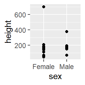
Figure 8.4: Woot! Data!
8.5.1.4 Munge inside ggplot
Ugh, crazy outliers, no grad student is ever that tall or short. Munge the data inside the ggplot function. On the fly!
ggplot(data = pcd %>%
         filter(height > 125 & height < 250),
       ) +
  geom_point(aes(x=sex, y=height))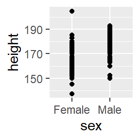
Figure 8.5: Fix the problem right in the data frame.
8.5.1.5 Try different geoms
Not a good use case for geom_point.
ggplot(data = pcd %>%
         filter(height > 125 & height < 250),
       aes(x=sex, y=height)) +
  geom_jitter()
## Warning in (function (kind = NULL, normal.kind = NULL, sample.kind = NULL) :
## non-uniform 'Rounding' sampler used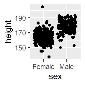
Figure 8.6: Try a different geom.
8.5.1.6 Customize the geom.
ggplot(data = pcd %>%
         filter(height > 125 & height < 250),
       aes(x=sex, y=height)) +
  geom_jitter(shape = 22, height = 0,
              width = 0.2, color = "blue",
              size = 4, alpha = 0.6)
## Warning in (function (kind = NULL, normal.kind = NULL, sample.kind = NULL) :
## non-uniform 'Rounding' sampler used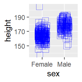
Figure 8.7: Let’s call this Bob-Rossing the plot.
8.5.1.7 Customize the axis labels
ggplot(data = pcd %>%
         filter(height > 125 & height < 250),
       aes(x=sex, y=height)) +
  geom_jitter(shape = 22, height = 0,
              width = 0.2, color = "blue",
               size = 4, alpha = 0.6)+
  # labs(title= "Precourse Survey",
  #      subtitle= "2014-2020",
  #      caption="IBS538 Spring 2020",
  #      tag = "Biostats",
  #      x="sex chromosome",
  #      y="verticality, cm")+
  scale_x_discrete(labels= c("XX", "XY"))
## Warning in (function (kind = NULL, normal.kind = NULL, sample.kind = NULL) :
## non-uniform 'Rounding' sampler used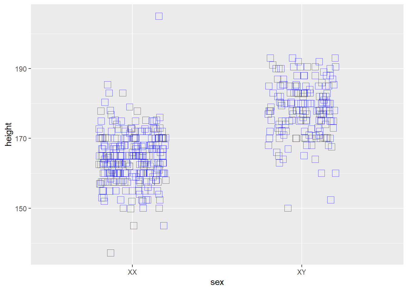
Figure 8.8: More Bob-Rossing.
8.5.1.8 Customize the frame & theme
ggplot(data = pcd %>%
         filter(height > 125 & height < 250),
       aes(x=sex, y=height)) +
  geom_jitter(shape = 22, height = 0,
              width = 0.2, color = "blue",
              size = 4, alpha = 0.6)+
  labs(title= "Precourse Survey",
       subtitle= "2014-2020",
       caption="IBS538 Spring 2020",
       tag = "Biostats",
       x="sex chromosome",
       y="verticality, cm")+
  scale_x_discrete(labels= c("XX", "XY"))+
  theme_classic()
## Warning in (function (kind = NULL, normal.kind = NULL, sample.kind = NULL) :
## non-uniform 'Rounding' sampler used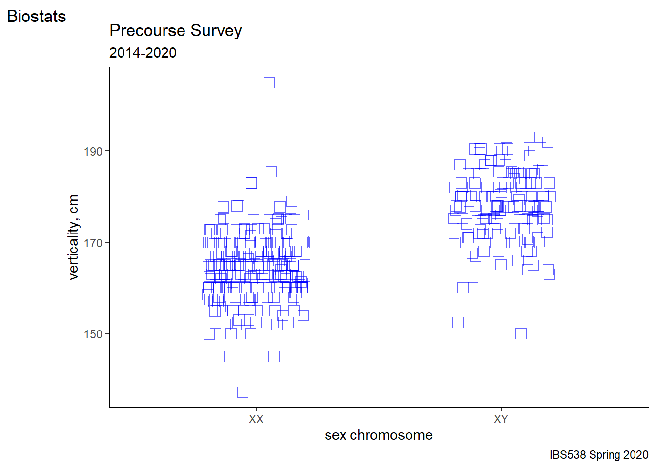
Figure 8.9: And more Bob-Rossing.
8.5.1.9 Add a third variable
The audience won’t “get” cm. Transform variable to inches. Oh, and segment using a third variable and applying scaling colors.
ggplot(data = pcd %>%
         filter(height > 125 & height < 250) %>%
         mutate(height = height/2.54),
       aes(x=sex, y=height, color = term)) +
  geom_jitter(shape = 18, height = 0,
              width = 0.2,
              size = 3, alpha = 1)+
  labs(title= "Precourse Survey",
       subtitle= "2014-2020",
       caption="IBS538 Spring 2020",
       tag = "Biostats",
       x="sex chromosome",
       y="verticality, INCHES")+
  scale_x_discrete(labels= c("XX", "XY"))+
  theme_classic()+
  scale_color_viridis(begin = 0.1, end =0.9)
## Warning in (function (kind = NULL, normal.kind = NULL, sample.kind = NULL) :
## non-uniform 'Rounding' sampler used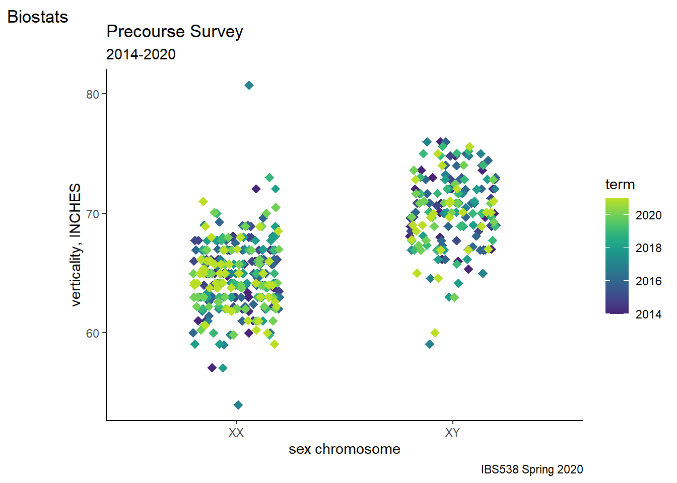
Figure 8.10: Finish with a dramatic combination data munge, Bob-Rossing flourish.
Much more could still be done, but I promised myself to stop at 10 steps. Start small, grow it. Play with it until you like it.
If that seems like a lot to code just for one figure, note that it is reproducible and modular. These latter features can be exploited with only slightly higher level R skills to repeatedly reuse the same custom format on many different data sets and variables.
8.6 Summary
This chapter focuses on the R you need for some of the assignments this week.
- Use R to inspect, modify and visualize variables.
- All R coding is like building a ggplot, through an iterative, step-by-step process.
- It pays to understand the starting material you have (data classification) to get the end product you want (summaries, plots and analysis).