Chapter 23 Rank Sum Distribution
The Wilcoxon rank sum per se represents a type of data transformation. The transformation is then used to calculate the nonparametric test statistic \(W\) for the Wilcoxon Test for independent two group samples, which is equivalent to the Mann-Whitney test. The distribution of \(W\) is discrete but normal-like.
Given two groups for comparison, such as a control population, \(X\) vs a treatment population, \(Y\). Under the null hypothesis, the distributions of the values of \(X\) and \(Y\) are equal.
Any effect due to treatment can be defined as \(\Delta = E(Y)-E(X)\), where \(E(Y)\) and \(E(X)\) are the averages for the treatment and control effects, respectively. Under the null hypothesis, \(\Delta = 0\).
23.0.1 Transformation of data into rank summs
\(X\) has a sample size \(m\) and \(Y\) has a sample size \(n\) and the total sample size is \(N=m+n\). Combine all values of \(X\) and \(Y\) and rank them from smallest to largest.
If \(S_1\) is the rank of \(y_1,..,S_n\) then W is the sum of the ranks assigned to the \(Y\) values: \(W=\sum_{j=1}^nS_j\)
23.0.2 The sign rank test statistic in R
When the null is true, the average of W is \(E_0(W)=\frac{n(m+n+1)}{2}\) and the variance is \(var_0(W)=\frac{mn(m+n+1)}{12}\). \(W\) can take on the values from zero to \(mn\).
23.1 R’s Four Sign Rank Distribution Functions
23.1.1 dwilcox
Given a value of \(W\) and group sample sizes \(m\) and \(n\), dwilcox will return the value of the probability for that \(W\). For example, here is the probability of getting a \(W\) of exactly 10 with group sizes of 5 and 6:
dwilcox(10, 5, 6)## [1] 0.04978355That probability is NOT a p-value. The p-value would be the sum of the probabilities returned from the dwilcox function for the range of \(W\) from 0 to 10.
Given the range of possible values for \(W\) its distribution can be plotted for any combination of group sizes. We can see that a value of 10 for \(W\) is left-shifted, but not too extreme.
m <- 5 #number of independent of group 1
n <- 6 #number of independent replicates of group 2
max <- m*n
df <- data.frame(pv=dwilcox(c(0:max), m, n))
ggplot(df, aes(x=c(0:max), pv)) +
  geom_col() + xlab("W") + ylab("p(W)")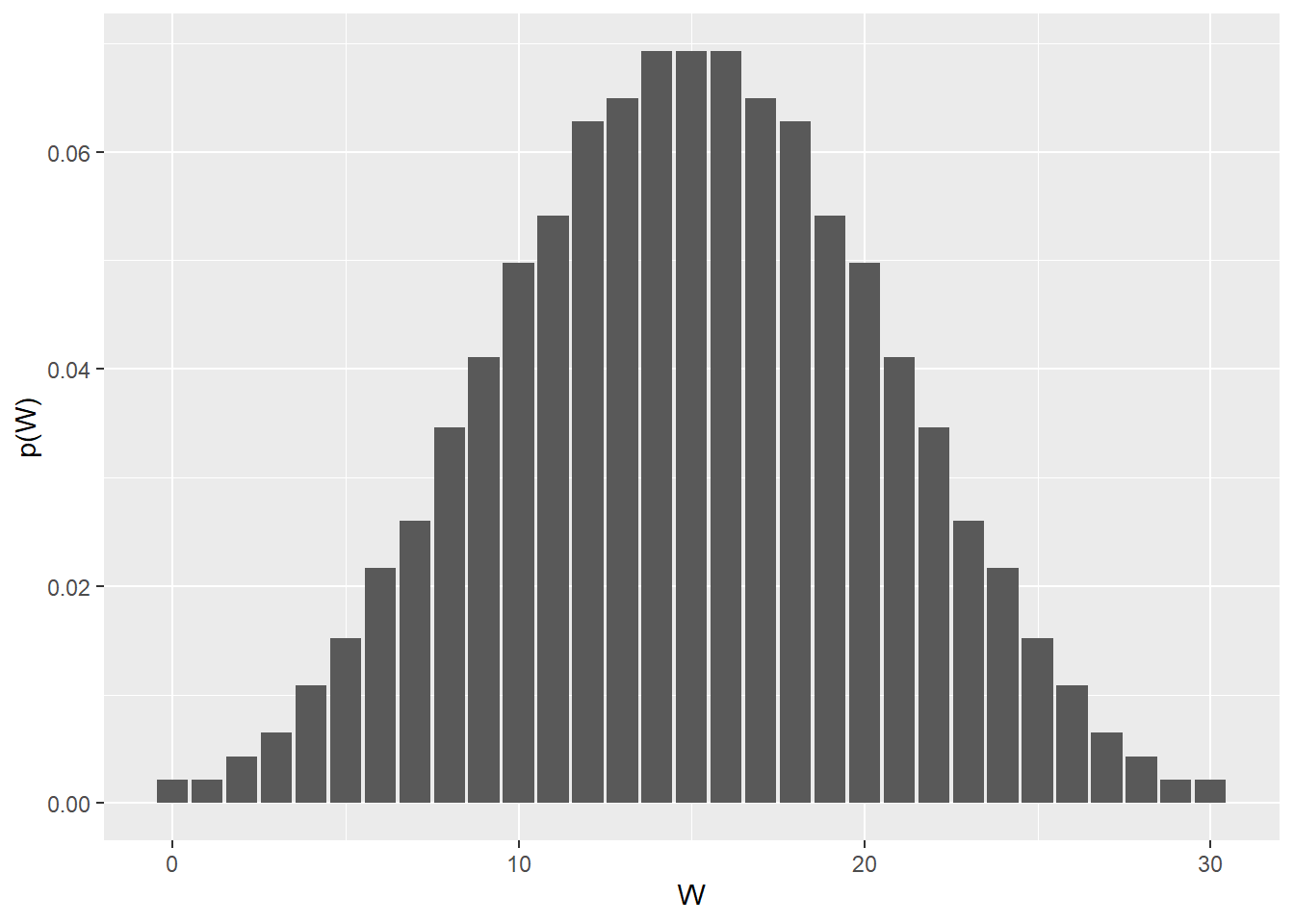
23.1.2 pwilcox
The pwilcox function returns a p-value when given \(W\) along with the sample sizes \(m\) and \(n\) corresponding to the two groups.
Thus, the probability of obtaining a \(W\) value of 10 or less with group sample sizes of 5 and 6 is:
pwilcox(10, 5, 6, lower.tail=T)## [1] 0.2142857The probability of obtaining a \(W\) value of 10 or more with group sample sizes of 5 and 6 is:
pwilcox(10, 5, 6, lower.tail=F)## [1] 0.7857143The relationship of pwilcox to dwilcox is as depicted here there is a slight inequality between the two functions somewhere beyond 10 significant digits, thus the rounding:
round(sum(dwilcox(c(0:10), 5, 6)), 10) == round(pwilcox(10, 5, 6), 10)## [1] TRUEHere are the lower and upper tailed cumulative distributions of the Wilcoxon distribution:
m <- 5
n <- 6
max <- m*n
df <- data.frame(pv=pwilcox(c(0:max), m, n))
ggplot(df, aes(x=c(0:max), pv)) +
  geom_col() + xlab("W") + ylab("p-value for W")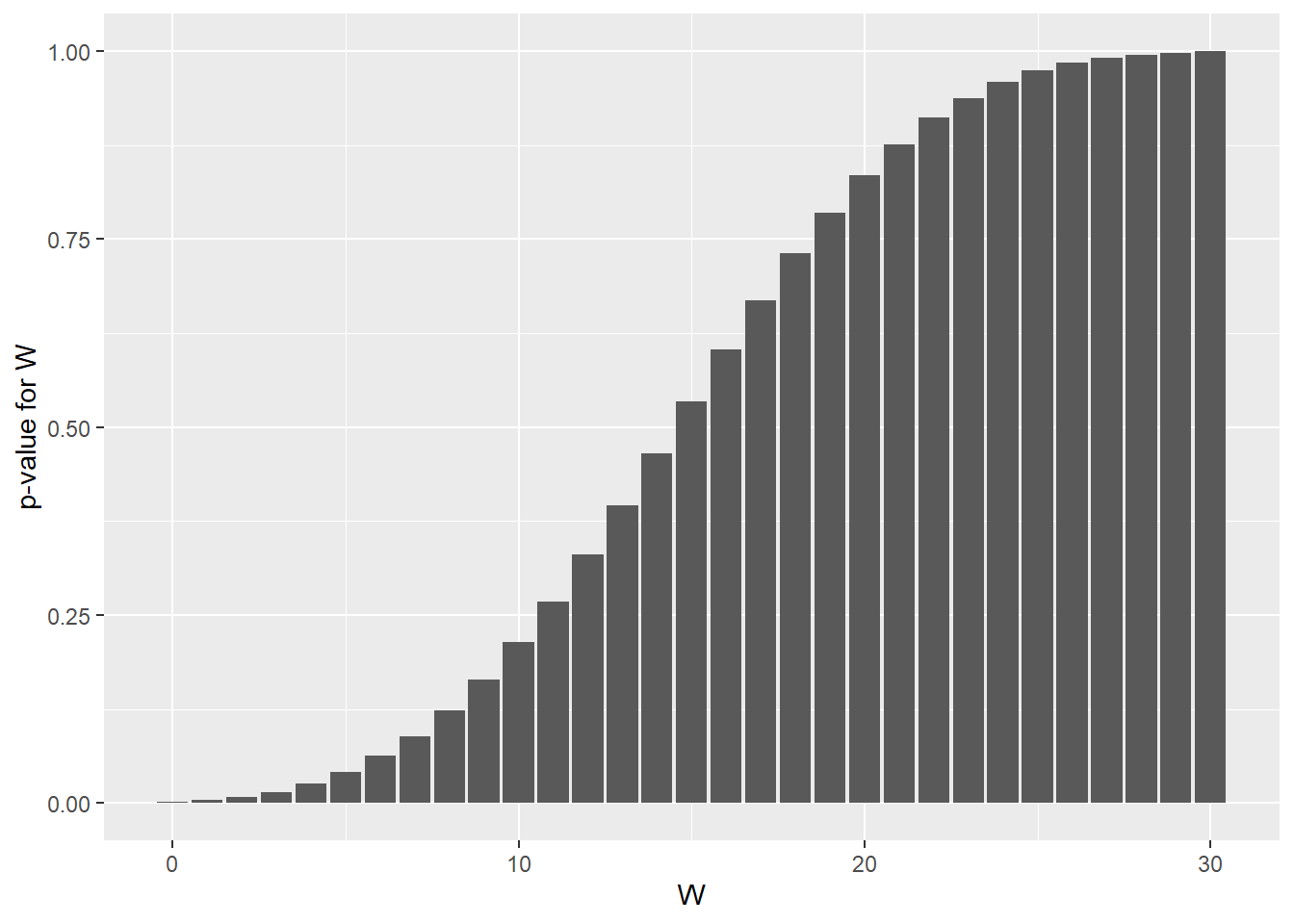
df <- data.frame(pv=pwilcox(c(0:max), m, n, lower.tail=F))
ggplot(df, aes(x=c(0:max), pv)) +
  geom_col() + xlab("W") + ylab("p-value for W")
23.1.3 qwilcox
This is the quantile signrank function in R. If given a quantile value (eg, 2.5%) and sample sizes \(m\) and \(n\), qwilcox will return the value of the corresponding test statistic \(W\).
For example, this can be used to find the critical limits for a two-sided hypothesis test for an experiment with 10 independent replicates, when the type1 error of 5% is evenly distributed to both sides:
qwilcox(0.025, 5, 6, lower.tail=T)## [1] 4qwilcox(0.025, 5, 6, lower.tail=F)## [1] 26Interpretation of critical limits output: When the null two-sided hypothesis is true, the values of \(W\) are \(4\le V\le26\). In other words, the null hypothesis would not be rejected if an experiment generated a \(W\) between 4 and 26.
Alternative interpretation: \(p<0.05\) when \(4>V>26\). In other words, a two sided null hypothesis would be rejected if it generated a \(W\) below 4 or greater than 26.
And here are the critical limits for one-sided hypothesis tests for an experiment with 10 independent replicates, when the type1 error is 5%. Notice how the critical limits differ between one-sided and two-sided tests:
qwilcox(0.05, 5, 6, lower.tail =T)## [1] 6qwilcox(0.05, 5, 6, lower.tail = F)## [1] 24Thus, having obtained a \(W\) of less than 6 or 24 and greater we would reject the null hypothesis. Do notice the distribution for these two sample sizes lacks perfect symmetry:
pwilcox(6, 5, 6)## [1] 0.06277056pwilcox(24, 5, 6, lower.tail=F)## [1] 0.04112554The quantile distribution of \(W\) is depicted below:
m <- 5
n <- 6
x <- seq(0,1,0.01)
df <- data.frame(w=qwilcox(x, m, n, lower.tail=T))
ggplot(df, aes(x=x, w)) +
  geom_point() + xlab("p-value") + ylab("W")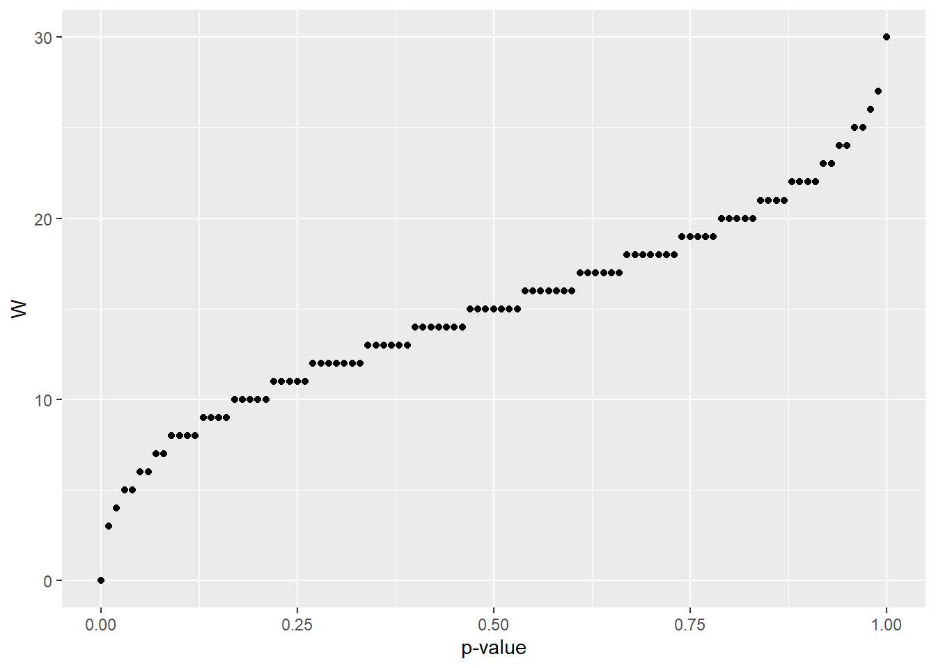
23.1.4 rwilcox
We would use rwilcox to generated random values of \(W\) from null distributions. Here are 7 random values of \(W\) for experiments involving sample sizes of \(m=5\) and \(n=6\)
rwilcox(7, 5, 6)## [1] 17 19 10 22 6 15 17Let’s simulate 1,000,000 such experiments. And then let’s count the number of extreme values of \(W\) that would randomly occur in that number of experiments.
We know from the qwilcox function that 24 is the critical value for a one-sided test at \(\alpha=0.05\).
Thus, our “significance test” for each of the 1,000,000 random experiments is to ask whether \(W\) is equal to or greater than 24.
Recall, the cumulative distribution function indicates the p-value for a one-sided test of a \(W=24\) is:
pwilcox(24, 5, 6, lower.tail=F)## [1] 0.04112554Given we’ve set a 5% false positive rate, we’d expect to see around 50000 false positives (5% of 1,000,000) by simulation of \(W=24\) under that scenario:
sim <- rwilcox(1000000, 5, 6)
test <- sim>=24
length(which(test==TRUE))
## [1] 62199In this instance, we see a much higher number of false positive 6.2% than the expected number of 5%! Why?