Chapter 31 One-way ANOVA Related Measures
library(tidyverse)
library(readxl)
library(viridis)
library(ez)
library(lme4)
The analysis, interpretation and presentation of a one-way ANOVA related/repeated measures experimental design is covered in this chapter.
This design has one predictor variable that is imposed at three or more levels.
But the essential feature of the RM design that distinguishes it from a CR design is that the measurements of the outcome variable are intrinsically related for all levels of the predictor within each independent replicate.
A complete experiment is therefore comprised of many independent replicates, within each of which are many intrinsically-linked measurements.
We’ll use data the Jaxwest2 study to illustrate this. In this example, growth of human tumors in immunodeficient mice is assessed by repeated measurements of tumor vol over a time period. Serial measurements in each of 11 independent replicates.
The outcome or dependent variable is tumor volume, in \(mm^3\). Tumor volumes are calculated after the researchers measured the lengths and widths of tumors using calipers.
The predictor variable is time, in units of days. Although time is usually a continuous/measured variable, we’ll treat it as a discrete factorial variable for this analysis.
The model organism is an immunodeficient mouse strain. Each mouse is an experimental unit that has been implanted with HT29 human colon tumor cells.
We imagine the experiment is designed to determine whether these cells will grow (rather than be rejected by the host immune system).
In truth, these are probably just control data from a contract test on an experimental drug or cancer treatment (the results of which are omitted).
The overall scope of the experiment is to test whether the immunodeficient mouse strain is suitable to study the properties of human cancers. A meaningful effect of the time variable in the ANOVA analysis implies that, yes, human tumors can grow in this host.
31.1 Data prep
The data are in a file called Jaxwest2.xls, which can be downloaded from the Jackson Labs here. That site offers more details about the study design than are listed here.
The munge has already been done conducted. For clarity, the script won’t be shown again here. However, it is used in this chapter to create a data frame object by the same name, jw2vol to be used for plotting and statistical analysis.
jw2 <-"datasets/jaxwest2.xls" %>%
  read_excel(
    skip=1,
    sheet=1
    )
# remove whitespace
names(jw2) <- str_remove_all(names(jw2)," ")


# trim columns
jw2vol <- jw2 %>%
  select(
    mouse_ID,
    test_group,
    contains("tumor_vol_")
    )

# trim cases
jw2vol <- jw2vol %>%
  filter(
    test_group == "Control (no vehicle)"
    )

# convert to numeric
jw2vol <- jw2vol %>%
  mutate_at(vars(tumor_vol_17:tumor_vol_44),
            as.numeric
            )
## Warning in mask$eval_all_mutate(quo): NAs introduced by coercion# impute
jw2vol <- jw2vol %>%
replace_na(
list(tumor_vol_17 =
mean(jw2vol$tumor_vol_17, na.rm=T)))
# pivot long
jw2vol <- jw2vol %>%
pivot_longer(cols=starts_with("tumor_vol_"),
names_to="day",
names_prefix = "tumor_vol_",
values_to = "vol"
)
# factorize
jw2vol <-jw2vol %>%
mutate(
mouse_ID=as.factor(mouse_ID),
test_group=as.factor(test_group)
)
jw2vol## # A tibble: 143 x 4
## mouse_ID test_group day vol
## <fct> <fct> <chr> <dbl>
## 1 38 Control (no vehicle) 17 27.2
## 2 38 Control (no vehicle) 18 54.8
## 3 38 Control (no vehicle) 19 77.6
## 4 38 Control (no vehicle) 22 104.
## 5 38 Control (no vehicle) 24 89.8
## 6 38 Control (no vehicle) 26 213.
## 7 38 Control (no vehicle) 29 306.
## 8 38 Control (no vehicle) 31 432.
## 9 38 Control (no vehicle) 33 743.
## 10 38 Control (no vehicle) 36 721.
## # ... with 133 more rows31.2 Data visualization
By the bloody obvious test it is clearly evident that tumor growth occurs in this model.
But here is the difficulty.
This is a repeated measures design. Tumor volume is measured on multiple days within each replicate.
The spaghetti plot and grouping by color illustrates the design of the experiment. The measurements within each color are intrinsically-liked. Not every point is an independent replicate. The number of independent replicates is far fewer. The number of colors is the number of independent replicates.
Plots like this show all of the data for an experiment.
ggplot(jw2vol, aes(as.numeric(day), vol, color=mouse_ID, group=mouse_ID))+
  scale_color_viridis(discrete=T)+
  geom_point(size=2)+
  geom_line()+
  xlab("Day after implant")+
  ylab("Tumor volume")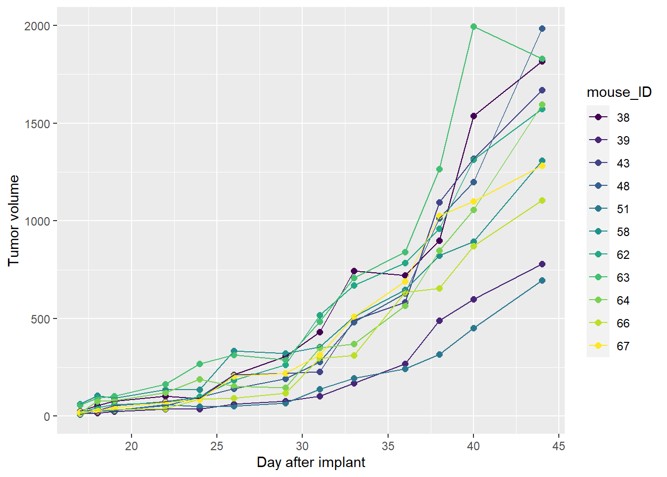
Figure 31.1: Tumor volume in each mose by days post transplantation
Statistically naive researchers would instead plot this as bar graphs. With group means by day, perhaps with bars with error. That visualization implies the means of the days matter, statistically. They do not.
The means of the slopes of the connecting lines between any two days are what matters statistically.
This looks swell. But not so fast.
31.2.1 Visualize the statistical design
The repeated measures statistical analysis operates not on group means, but on the means of differences between levels of a factor, in the same way a paired t-test is about the difference between treatment effects.
The following illustrates this.
The code below calculates the difference in tumor volume within each mouse between successive days. For example, for mouse #38, the day 40 volume is subtracted from day 44, 38 from 40, 36 from 38, and so on. The function lag helps do this automagically.
sum <- jw2vol %>%
  # ensure sequential
  mutate_at(vars(day), as.numeric) %>%
  group_by(mouse_ID) %>%
  mutate(diff=vol-lag(vol, default=first(vol)))
We might be interested in those differences between two sequential measurement days for scientific reasons. For example, it might be useful for detecting a significant acceleration in tumor growth.
ggplot(sum, aes(day, diff, color = as.factor(mouse_ID)))+
  scale_color_viridis(discrete=T)+
  geom_hline(aes(yintercept=0),
             color="blue", size=0.5,
             linetype="dashed")+
  scale_y_continuous(limits=c(-250, 1000))+
  stat_summary(fun.data=mean_sdl, fun.args = list(mult=1),
                 geom="errorbar", color="blue")+
  stat_summary(fun.y=mean, geom="point", color="blue")+
  geom_point(size=3)+
  xlab("Lead day")+
  ylab("Tumor vol difference \n (diff::lead day - lag day)")+
  labs(color ="mouse_id")
## Warning: `fun.y` is deprecated. Use `fun` instead.## Warning: Computation failed in `stat_summary()`:
## Can't convert a double vector to function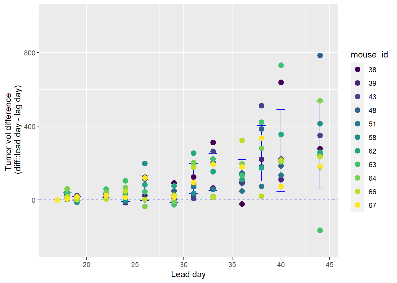
Figure 31.2: Differences in tumor volume from prior measurement in each mouse.
Alternately, we might be interested in the earliest detectable difference in tumor growth relative to, for example, the first day of measurements. At what point is it clear the tumore is growing? Here are the mean differences within the mice from each day of measurement back to the volume measured on day 17.
This is the type of analysis we would do for repeated measure data rather than the Dunnett’s test, which is for unpaired comparisons.
sum2 <- jw2vol %>%
  # ensure sequential
  mutate_at(vars(day), as.numeric) %>%
  group_by(mouse_ID) %>%
mutate(diff=vol-first(vol))ggplot(sum2, aes(day, diff, color = as.factor(mouse_ID)))+
scale_color_viridis(discrete=T)+
geom_hline(aes(yintercept=0),
color="blue", size=0.5,
linetype="dashed")+
scale_y_continuous(limits=c(-250, 2000))+
stat_summary(fun.data=mean_sdl, fun.args = list(mult=1),
geom="errorbar", color="blue")+
stat_summary(fun.y=mean, geom="point", color="blue")+
geom_point(size=3)+
xlab("Lead Day")+
ylab("Tumor vol difference \n (diff::lead day - first day)")+
labs(color ="mouse_id")## Warning: `fun.y` is deprecated. Use `fun` instead.## Warning: Computation failed in `stat_summary()`:
## Can't convert a double vector to function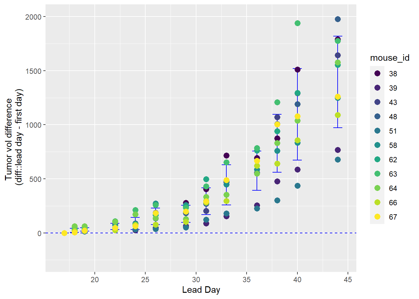
Figure 31.3: Differences in tumor volume from day 17 measurement in each mouse.
31.3 The ANOVA
Every ANOVA test is one-sided. They test whether the variance associated with the model is greater than the variance associated with the residual error. To test the null, \[H_0: \sigma^2_{model}\le\sigma^2{residual}\]
What is the model in this case?
All of the variation in tumor_vol variable can be accounted for by this relationship:
\[SS_{total}=SS_{day}+SS_{mouseID}+SS_{residual}\]
We have 143 volume measurements in the data set. But they don’t come, once each, from 143 different mice. Since we take repeated measures from each of 11 mice we can account for the variation associated within the mice. That’s basically variation that would otherwise have been in the residual term. Since we can account for it, we can put in our model term.
\[SS_{model}=SS_{day}+SS_{mouseID}\] and so \[SS_{total}=SS_{model}+SS_{residual}\]
Variance is just the \(SS\) averaged using the degrees of freedom. For our experiment, the F statistic is ratio of the model in the numerator to the residual variance in the denominator,
\[F=\frac{\frac{SS_{model}}{df_n}}{\frac{SS_{residual}}{df_d}}\]
31.3.1 Running ezANOVA
Running the function is ezANOVA function straightforward. Configuring it as below ensures that the \(SS\) associated with the mouse_ID term gets partitioned out of the residual and into the model.
The data have been munged previously into the data frame jw2vol. See above and here.
Because this involves repeated measures for each mouse, the time variable day is argued as within. We might say, “the tumor_vol measurements are repeated within the day variable.”
The combination of the wid=mouse_ID and the within = mouse_ID arguments are what ensures the function knows this is a RM on day design.
Type 1 sum of squares is chosen for this calculation only because a type 2 calculation produced a computation error. This is not a concern since this is a one-way ANOVA.
Strictly, we ask does “day” have any influence on tumor growth?
A detailed ANOVA table is called. There are additional arguments that could be made for custom situations. Consult ?ezANOVA for more information.
There are a few ways to output the analysis. Here’s the simplest:
one_wayRM <- ezANOVA(data = jw2vol,
                     dv = vol,
                     wid = mouse_ID,
                     within = day,
                     detailed=T,
                     type=1)
one_wayRM
## $ANOVA
## Effect DFn DFd SSn SSd F p p<.05 ges
## 1 day 12 120 27138034 3115733 87.09999 2.830845e-53 * 0.897013431.4 Interpretation
The effect reminds us that the model is day. The inclusion of the mouse_ID in the model is not reported from this particular function. But we can tell this is properly accounted by the degrees of freedom values.
DFn is the degrees of freedom for the F test numerator. This is one less than number of levels (13) in the day variable.
DFd is the degrees of freedom for the F test denominator. We have 143 measurements and begin with 143 degrees of freedom. We lost one degree of freedom for the grand mean. We also remove from the residuals the 12 degrees of freedom for the day variable. We also have 11 mouses, comprising 10 degrees of freedom that are also in the model. That leaves 120 df for the residual error.
SSn is \(SS_{model}\). SSd is \(SS_{residual}\). Divide each of those by their respective degrees of freedom and you have two variances.
F is the ratio of the variances, \[F_{DFn,DFd}=\frac{\frac{SSn}{DFn}}{\frac{SSd}{DFd}}\]
This F-statistic tests the null hypothesis, which is that the variation associated with day+mouse_id is less than or equal to or less than residual variation. The experimental F is tested against an F distribution with 12 and 120 degrees of freedom.
The p-value is the probability of obtaining an F-statistic value this high or even more extreme if the null hypothesis were true. When this value is less than a predetermined type1 error threshold the null can be safely rejected.
The ges is a regression coefficient ‘general eta squared’ that can take on values between 0 and 1. It is analogous to the better known regression coefficient \(R^2\)
GES is the ratio of the variation due to the effect of the model to the total variation in the data set: \[ges=\frac{SS_{model}}{SS_{residual}+SS_{model}}\] The value of 0.897 can be interpreted as follows: 89.7% of the observed variation in the data is associated with the differences between days when controlled for mouse_ID.
Scientifically, you can infer from this F-test result that the HT29 tumor volumes grow with time when implanted into this mouse strain.
Sometimes, that’s all you wish to conclude. Does the tumor injection model work with this strain and that tumor cell line? Yes. End of story.
If we wish to further identify differences of scientific interest we could do a post-hoc analysis. We are under no obligation to do so.
31.5 Post-hoc analysis
I have a fairly extensive discussion elsewhere about posthoc analysis. See Chapter 35.
Note that since this is a related measures ANOVA I recommend not using range tests (eg, Dunnett’s or Tukey, etc) since those operate on group means. Related measures deals with paired measures and the posthoc questions are whether the mean of the differences between paired measures is zero. Therefore, there is no discussion of range tests below.
Perhaps we’d like to dig a little deeper. For example, we might want to know on which days tumor growth differs from the first day in the recorded series of measurements.
The approach taken below involves two steps.
First, all pairwise comparisons are made using a paired t-test to generate a matrix of all unadjusted p-values.
Second, a vector of select p-values will be collected from this matrix. These p-values will then passed into the p.adjust function so that they are adjusted for a fewer number of multiple comparisons.
First, the pairwise t-test. Note the arguments. No adjustment is made (yet) and a two-sided paired t-test is called. The output of the function is stored in an object named m.
jw2vol <-jw2vol %>%
  mutate(
    day=as.factor(day)
    )

m <- pairwise.t.test(x = jw2vol$vol,
                     g = jw2vol$day,
                     p.adjust = "none",
                     paired = T,
                     alternative = "two.sided"
                     )
m
##
## Pairwise comparisons using paired t tests
##
## data: jw2vol$vol and jw2vol$day
##
## 17 18 19 22 24 26 29 31 33
## 18 0.00181 - - - - - - - -
## 19 6.8e-05 0.02302 - - - - - - -
## 22 4.0e-05 3.7e-05 0.00026 - - - - - -
## 24 0.00042 0.00080 0.00235 0.02637 - - - - -
## 26 6.4e-05 0.00012 0.00019 0.00056 0.00985 - - - -
## 29 2.3e-05 4.8e-05 5.3e-05 0.00023 0.00489 0.06577 - - -
## 31 1.4e-05 1.6e-05 1.7e-05 3.7e-05 6.0e-05 0.00078 0.00083 - -
## 33 1.3e-05 1.7e-05 1.6e-05 2.4e-05 4.1e-05 3.6e-05 1.8e-05 0.00053 -
## 36 1.0e-06 1.1e-06 1.1e-06 1.6e-06 1.3e-06 1.3e-06 1.0e-06 8.6e-07 0.00058
## 38 1.3e-06 1.5e-06 1.4e-06 1.6e-06 1.2e-06 1.1e-06 1.6e-06 7.1e-06 1.4e-05
## 40 6.3e-06 6.9e-06 6.6e-06 7.3e-06 6.0e-06 8.0e-06 8.9e-06 1.4e-05 1.3e-05
## 44 7.0e-07 7.0e-07 6.9e-07 7.6e-07 6.5e-07 7.8e-07 7.1e-07 1.1e-06 8.6e-07
## 36 38 40
## 18 - - -
## 19 - - -
## 22 - - -
## 24 - - -
## 26 - - -
## 29 - - -
## 31 - - -
## 33 - - -
## 36 - - -
## 38 0.00023 - -
## 40 0.00014 0.00247 -
## 44 4.5e-06 1.1e-05 0.00181
##
## P value adjustment method: noneThe pairwise.t.test output m is a list of 4 elements.
str(m)## List of 4
## $ method : chr "paired t tests"
## $ data.name : chr "jw2vol$vol and jw2vol$day"
## $ p.value : num [1:12, 1:12] 1.81e-03 6.84e-05 4.05e-05 4.18e-04 6.40e-05 ...
## ..- attr(*, "dimnames")=List of 2
## .. ..$ : chr [1:12] "18" "19" "22" "24" ...
## .. ..$ : chr [1:12] "17" "18" "19" "22" ...
## $ p.adjust.method: chr "none"
## - attr(*, "class")= chr "pairwise.htest"The most important of these is $p.value, which you can see is a matrix.
class(m$p.value)## [1] "matrix" "array"The matrix contains p-values that represent the outcome of paired t-tests for tumor_vol between all possible combinations of days.
Thus, the p-value in the cell defined by the second row and second column of the matrix (m$p.value[2,2]=0.00182) reflects that for the mean difference in tumor_vol between the 17th and 18th days. (note: day 22 is out of order)
The first column of p-values, m$p.value[,1], are paired t-test comparisons of tumor_vol between the 22th day and each of the days 18 through 44.
pv <- m$p.value[,1]
pv
## 18 19 22 24 26 29
## 1.813199e-03 6.836240e-05 4.047601e-05 4.184046e-04 6.397132e-05 2.285676e-05
## 31 33 36 38 40 44
## 1.434113e-05 1.320992e-05 1.030436e-06 1.298778e-06 6.341427e-06 7.020905e-07To create the adjusted p-values, we pass the vector of p-values pv selected from the p-value matrix m into the p.adjust function. Use your judgement to select an adjustment method that you deem most appropriate.
p.adjust(p = pv,
         method = "bonferroni",
         n = length(pv)
         )
## 18 19 22 24 26 29
## 2.175839e-02 8.203488e-04 4.857121e-04 5.020856e-03 7.676558e-04 2.742811e-04
## 31 33 36 38 40 44
## 1.720936e-04 1.585190e-04 1.236523e-05 1.558534e-05 7.609713e-05 8.425086e-06Since each of these adjusted p-values is less than the type 1 error threshold of 0.05, we can conclude that the mean difference in tumor volume changes on each day through the study. If we were one to to put asterisks on the figure, we would illustrate one for each of the days (other than day 17).
31.6 Write up
Here’s how we might write up the statistical methods.
For the jaxwest2 experiment, each of 11 mice are treated as independent replicates. Repeated tumor volume measurements were collected beginning on day 17 post-implantation. The tumor volume value for day = 17 for the 3rd subject was lost. This was imputed using the average tumor volume value for day 17 of all other subjects. The effect of time was assessed by one-way repeated measures ANOVA with type 1 sums of squares calculation. For a post hoc analysis, the mean differences in tumor vol between study days were compared using two-sided paired t-tests (pairwise.t.test), with p-values adjusted using the Bonferroni method.
In the figure legend, something like this:
Tumor volume increases with days after implantation (one-way RM ANOVA, F(12,120)=87.1, p=2.8e-53). Asterisks = adjusted p < 0.05.