Chapter 45 Logistic regression
Sometimes our experiments generate discrete outcome responses as either of two conditions: yes or no, up or down, in or out, absent or present, sick or healthy, pregnant or not, alive or dead.
You get the idea. An event can either not happen, or it can happen.
Since the beginning of this course we’ve been calling these “sorted” outcome variables. Other commonly used jargon refers to these as nominal, dichotomous, binary or binomial.
To recall, proportions are the number of “successes” or events in a trial of size \(n\). Proportions take on the values from 0 to 1. A given proportion can serve as a point estimate of the sampled population. In a long run the proportion has some probability between the extremes of 0 and 1, which can be modeled using the binomial distribution.
We discuss the statistical treatment of sorted data in Chapter 19 for relatively simple experimental designs involving one or two levels of a predictor variables. For example, the proportion of cells that survive after exposure to a toxin compared to a control. Or the proportion of cells on a dish in which the nuclei are stained positive for an antigen after a stimulus, compared to a control.
Logistic regression extends proportion analysis. It provides a way to analyze data sets in which more than two proportions must be evaluated simultaneously or for when the response is binary over a range of predictor values.
We’re now at the point where we’re able to close a loop of sorts. If you recall from way back at the beginning of the course, we dealt with tests that compare two proportions. In other words, we were only equipped to perform experiments comparing two groups. Now that we are more knowledgeable about regression techniques, we can apply regression to deal with more than two proportions.
For measured outcome data, we have t-tests to compare two or fewer groups, but then acquired facility using ANOVA and linear regression (or multiple linear regression) for experiments with more than two groups to compare.
For ordered outcome data, we have sign rank and rank sum tests for two samples or less, and have Kruskal Wallis or Friedman’s test for more groups to compare.
With logistic regression we can now analyze experiments that produce sorted outcome responses and that involve more than two groups of predictors!
45.1 Uses of logistic regression
Use logistic regression when an outcome is a nominal categorical variable and for
- isolating the influence of individual variables on a response.
- predicting the odds and probability of a response.
- measuring the interplay of multiple variables in a response.
- making inferential decisions about whether a predictor causes a response.
45.2 Derivation of the logistic regression model
A simple linear model for an event probability in response to a continuous explanatory variable \(X\) has the form \(Y=\beta_0 +\beta_1X + \epsilon\), where \(Y\) is a probability that can only take on values \(0\le P\le 1\). For now, we’ll dismiss random error to simplify. It can be shown that in order for \(Y\) to meet the latter condition the following proportion is true
(equation 1) \[P(Y=1|X)=\frac{exp(\beta_0 +\beta_1X)}{exp(\beta_0+\beta_1X)+1}\]
That relationship can be transformed algebraically to express the odds of an event, \(\frac{p}{1-p}\), as an exponential function
(equation 2) \[\frac{p}{1-p}=exp(\beta_0+\beta_1X)\], which when transformed using the natural logarithm becomes a linear function on X.
(equation 3) \[log(\frac{p}{1-p})=\beta_0+\beta_1X\].
The left-sided term \(log(\frac{p}{1-p})\) is referred to as the ‘logit’ or as ‘log odds.’ It represents, of course, the natural logarithm of the odds. Transforming eq3 using the exponential generates eq2.
45.2.1 Relationship of logit to odds to the model coefficients and probability
Probabilities can be calculated from odds following exponential transformation of logit. Thus, for a linear logistic model:
(equation 4) \[odds=exp(logit)=exp(\beta_0+\beta_1X)\] (equation 5) \[p=\frac{odds}{odds+1}\] (equation 6) \[for\ one\ coefficient, e.g: odds=exp(\beta)\] (equation 6) \[percent \ change=(odds-1)*100\]
45.2.1.1 Graphical relationships between proportions, odds and logit
Sometimes it’s helpful to visualize the relationships between these parameters graphically.
The first graph, which is on a linear scale, illustrates how odds are an exponential function of probability. The second graph is on a semi-log scale. Log transformation of odds yields logit, which has a log-linear relationship with probability.
a <- seq(99, 1, -1)
d <- seq(1, 99, 1)

p <- a/(a+d)
odds <- p/(1-p)
logit <- log(p/(1-p))

ggplot()+
  geom_point(aes(p, odds))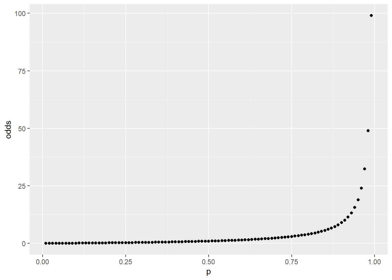
Figure 45.1: Odds are an exponential function of probability.
ggplot()+
  geom_point(aes(p, logit))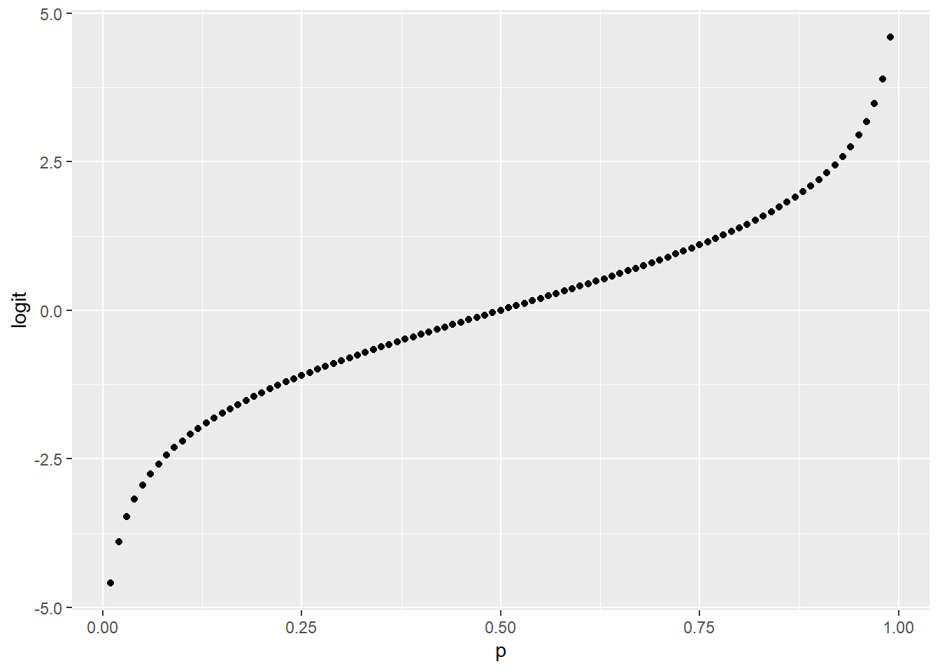
Figure 45.2: Odds are an exponential function of probability.
The graph below provides, I think, the most intuitive way to think about what logit values mean. Their relationship to probability is almost switch-like. For example, a log odds value of 3 indicates that an outcome is highly probable.
logit <- seq(-6, 6, 1)

p <- exp(logit)/(1+exp(logit))

ggplot()+
  geom_point(aes(logit, p))+
  scale_x_continuous(breaks = -6:6)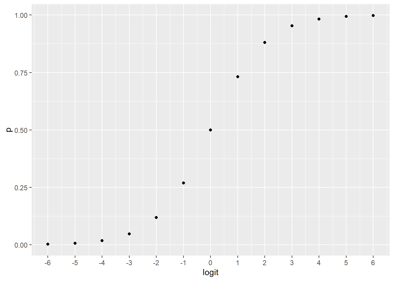
Figure 45.3: Changing the axis illustrates the nonlinear switch-like relationship between logit and probability.
45.2.2 Additional types of logistic regression models
Logistic regression can be adapted to virtually any other experimental design described by a general linear model, a few examples are listed below.
45.2.2.1 one factorial explanatory variable
\(ln(\frac{p}{1-p})=\beta_0+\beta_1 A\)
45.2.2.2 two factorial explanatory variables
\(ln(\frac{p}{1-p})=\beta_0+\beta_1 A+\beta_2 B\)
45.2.2.3 multiple explanatory variables of any type
\(ln(\frac{p}{1-p})=\beta_0+\beta_1X_1+\beta2X_2..+\beta_nX_n\)
45.2.2.4 Running logistic regression in R
So as you can see, at a higher level, logistic regression is not really different than linear regression modeling.
The model options determined by the predictor variables in the study. The right hand of the equation is some general linear model that accounts for the predictor variable(s) of your experiment. The left hand of the left hand of the equation is logit.
We use the glm() function in R rather than the lm() function. The reason for that is logistic regression is a type of generalized linear model. These models “generalize” nonlinear functions (such as logit) as linear models.
In linear and nonlinear regression (and also t-tests and ANOVA) model variation is accounted for using ordinary least squares (OLS) estimation. OLS serves as a common statistical thread that ties together the various parametric techniques, from t-tests to more complex nonlinear regression models and multiple regression.
Instead of OLS, generalized linear models such as logistic regression use maximum likelihood estimation (MLE) to derive parameter values. MLE generates parameter value estimates through iterative calculations that maximize the likelihood the regression model produced the data that were actually observed.
Why MLE and not OLS? The short answer is that generalized linear models are frequently used on data that violate the assumptions for valid use of OLS-based statistical methods. Logistic regression is a perfect example: OLS has no utility in the analysis of binary outcomes!
45.3 Stress and survival
Blas(2007) measured plasma corticosterone(ng/ml) in nestling storks after inducing an experimental stress. The birds were then followed over 5 years, and recorded as either survived (0) or dead (1) by the end of that period. By convention, a value of 1 is assigned to “events” and 0 assigned to “nonevents” for binary outcome data. In this instance, an event was death.
It is VERY important to recognize that every stork is statistically independent of every other stork. The experiment below has 34 independent replicates.
Note how the outcome variable, death, is comprised of zeroes and ones. Nonevents and events.
The variable cort is measured corticosterone levels in nestlings after they had received a stress. But it is used here as a predictor variable. It serves as an index of the severity induced in each nestling treatment. A common stress treatment delivered to each nestling is refactored to a continuous predictor variable that signals the impact of that treatment.
cort <- c(26,28.2,29.8,34.9,34.9,35.9,37.4,37.6,38.3,39.9,41.6,42.3,52,26.6,27,27.9,31.1,31.2,34.9,35.9,41.8,43,45.1,46.8,46.8,47.4,47.4,47.7,47.8,50.7,51.6,56.4,57.6,61.1)

death <- c(1,1,1,1,1,1,1,1,1,1,1,1,1,0,0,0,0,0,0,0,0,0,0,0,0,0,0,0,0,0,0,0,0,0)

stork <- data.frame(cort, death)

ggplot(stork, aes(cort, death))+
  geom_point(shape=1, size=8, color="blue")+
  labs(y="P(dead)", x="corticosterone, ng/nl")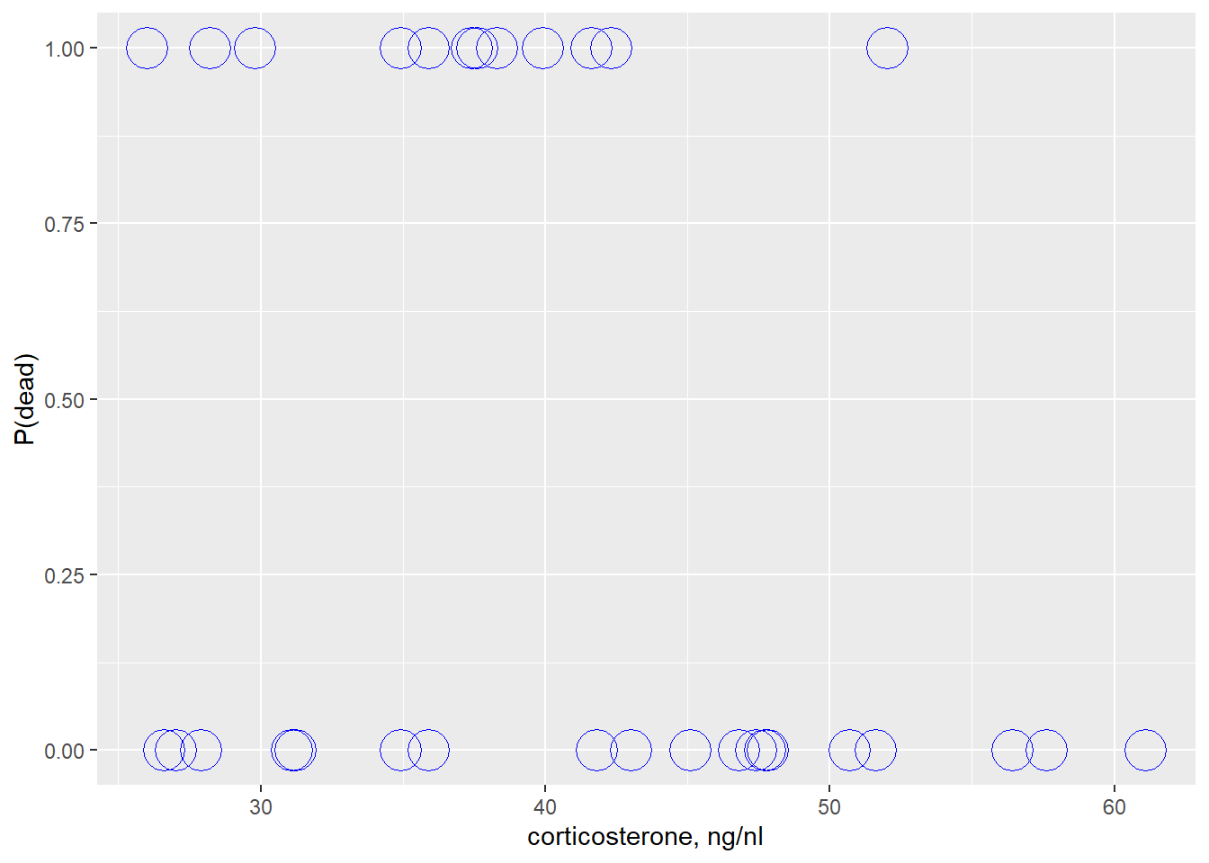
This plot can be a bit disorientating. Remember, deaths are events and so are assigned a value of 1. If you assume higher cortisol is proportional to stress intensity experienced by the birds, a quick glance suggests higher early stress events offer a survival advantage.
Given the nature of the binary response variable, we can model it logistically as such: \[logit(survive)=\beta_0+\beta_1(cort)\]
Let’s run a quick linear regression.
We use glm because we can’t use lm on binomial response data, and we need to tell it what family of data for the dependent variable (response) to model.
stork.model <- glm(death~cort, family=binomial(), stork)
summary(stork.model)
##
## Call:
## glm(formula = death ~ cort, family = binomial(), data = stork)
##
## Deviance Residuals:
## Min 1Q Median 3Q Max
## -1.4316 -0.8724 -0.6703 1.2125 1.8211
##
## Coefficients:
## Estimate Std. Error z value Pr(>|z|)
## (Intercept) 2.70304 1.74725 1.547 0.1219
## cort -0.07980 0.04368 -1.827 0.0677 .
## ---
## Signif. codes: 0 '***' 0.001 '**' 0.01 '*' 0.05 '.' 0.1 ' ' 1
##
## (Dispersion parameter for binomial family taken to be 1)
##
## Null deviance: 45.234 on 33 degrees of freedom
## Residual deviance: 41.396 on 32 degrees of freedom
## AIC: 45.396
##
## Number of Fisher Scoring iterations: 445.3.1 Interpretation of output
First, let’s try to make sense of this graphically.
Using augment from the broom package is a nifty way to see the predicted values of the fitted model. We’ll plot those out three different ways below to visualize the survival response to stress levels. In each graph, the fitted values of the model are used. They’re just transformed in the latter two.
augment(stork.model)## # A tibble: 34 x 8
## death cort .fitted .resid .std.resid .hat .sigma .cooksd
## <dbl> <dbl> <dbl> <dbl> <dbl> <dbl> <dbl> <dbl>
## 1 1 26 0.628 0.925 0.978 0.106 1.14 0.0353
## 2 1 28.2 0.453 0.992 1.04 0.0868 1.14 0.0331
## 3 1 29.8 0.325 1.04 1.08 0.0740 1.14 0.0312
## 4 1 34.9 -0.0821 1.21 1.24 0.0432 1.13 0.0256
## 5 1 34.9 -0.0821 1.21 1.24 0.0432 1.13 0.0256
## 6 1 35.9 -0.162 1.25 1.27 0.0395 1.13 0.0251
## 7 1 37.4 -0.282 1.30 1.32 0.0355 1.13 0.0253
## 8 1 37.6 -0.298 1.31 1.33 0.0352 1.13 0.0254
## 9 1 38.3 -0.353 1.33 1.35 0.0341 1.13 0.0260
## 10 1 39.9 -0.481 1.39 1.41 0.0333 1.13 0.0288
## # ... with 24 more rowsA plot of the fitted linear model values in units of logit onto the corticosterone scale. The plot is, of course, linear. The ordinate is scale logit or log odds. Logit is not particularly intuitive unless you use it a lot.
ggplot(augment(stork.model), aes(cort, .fitted))+
  geom_point()+
  ylab(".fitted aka logit")+
  ggtitle("logit=2.703-0.0798*cort")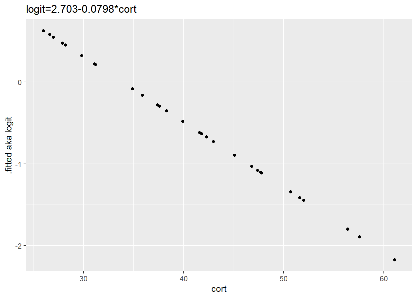
Next, we’ll rescale the fitted values as odds through taking the exponent on both sides. The graph’s ordinate is now in units of odds. Recall, odds are the ratio of the probability of an event to its complement.
The result is an exponential relationship, negative in this case. The odds of stork death drop with the magnitude of nestling corticosterone (as a stress marker).
ggplot(augment(stork.model), aes(cort, y=exp(.fitted)))+
  geom_point()+
  ylab("exp(.fitted) aka odds")+
  ggtitle("odds=exp(2.703-0.0798*cort)")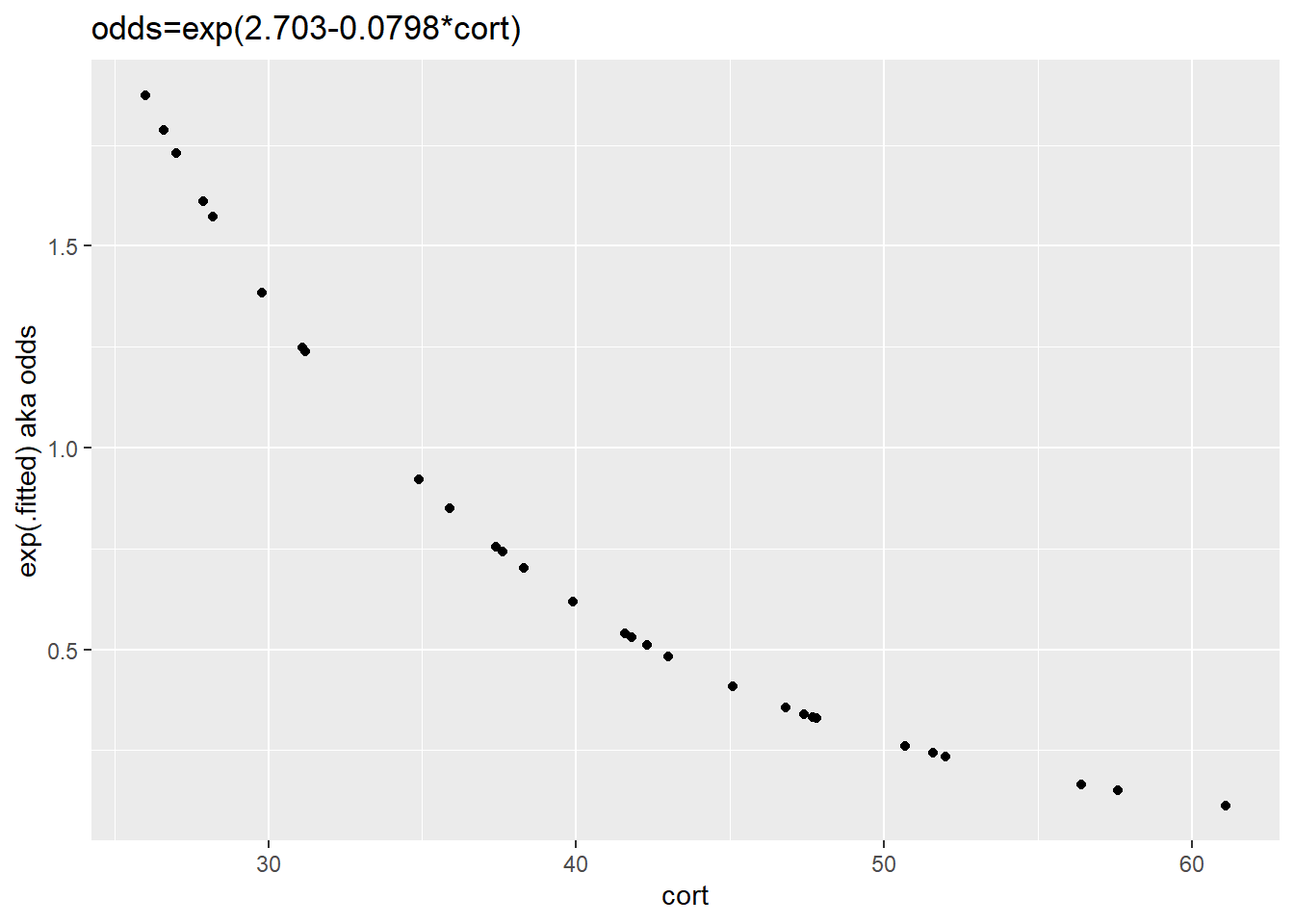
Lastly, we’ll transform the fitted values to probabilities. This also happens to be the scale of the original data, so we’ll add those experimental values to the fitted values. The fitted values are nonlinear on this scale, an S-shaped curve is ever-so-faint. The probability of death is reduced as stress levels increase.
ggplot(augment(stork.model), aes(cort, y=exp(.fitted)/(exp(.fitted)+1)))+
  geom_point()+
  ylab("odds/odds+1 aka P(death)")+
  ggtitle("P=exp(2.703-0.0798*cort)/exp(2.703-0.0798*cort)+1")+
  geom_point(data=stork, aes(y=death), shape=1, size=8, color="blue")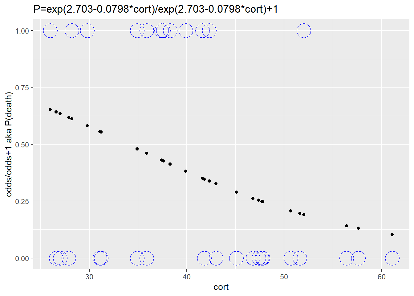
45.3.1.1 Coefficient values
kable(tidy(stork.model))| term | estimate | std.error | statistic | p.value |
|---|---|---|---|---|
| (Intercept) | 2.7030391 | 1.7472461 | 1.547028 | 0.1218564 |
| cort | -0.0798047 | 0.0436801 | -1.827025 | 0.0676959 |
The coefficient estimates and standard error values are derived from maximum likelihood estimation. They are linear model parameteres that, generally, predict the linear relationship between X and Y, where the latter is in logit units. In this case, the fixed coefficients between nestling stress (corticosterone) and the log odds of death.
Bear in mind that Y is logit, or log-odds units, allows for linearization of a nonlinear phenomenon and may not be intuitively useful. Nevertheless, plugging the coefficient values into the formula the linear model for the data is \(logit(Y)=2.7030-0.0798*X\)
It can be more interpretable to convert from log-odds to odds or to proportions.
To convert log-odds to ordinary proportions we use equation 1 above. For example, what proportions of storks with a corticosterone level of 30 or 60 ng/ml are predicted to die?
#let `l` be our linear model
c <- c(30, 60)
l <- 2.7030-0.0798*c
p <- exp(l)/(exp(l)+1)
p
## [1] 0.5766412 0.1105633Thus, a 57.7% death rate is predicted for nestling stress corresponding to cort levels of 30 ng/ml. Doubling the stress reduced the death rate to 11%.
The coefficients allow for predicting the fractional contribution of a unit change in level of the explanatory variable:
\(percent \ change=(logit-1)*100\) or \(percent \ change=(odds-1)*100\)
For example, by what percent does a 1 ng/ml increase in cort change the odds of survival?
To calculate in terms of odds, note how we do an exponential transform of the value of the coefficient from log-odds to odds:
(exp(-0.0798)-1)*100## [1] -7.669901Thus, a 1 ng/ml increase in cort would be associated with a 7.67% decrease in death.
If we’d like to have confidence intervals, in logit units, those are easy to compute:
confint(stork.model)## Waiting for profiling to be done...## 2.5 % 97.5 %
## (Intercept) -0.5583249 6.434585e+00
## cort -0.1746984 2.847104e-0545.3.1.2 Deviance
The regression model includes the calculation of two deviance values:
kable(glance(stork.model))| null.deviance | df.null | logLik | AIC | BIC | deviance | df.residual | nobs |
|---|---|---|---|---|---|---|---|
| 45.23389 | 33 | -20.69785 | 45.3957 | 48.44843 | 41.3957 | 32 | 34 |
The term ‘deviance’ signals that maximum likelihood estimation is used in these calculations. As you might imagine, deviance residuals are analogous to residuals calculated using ordinary least squares. Deviance represents the deviation from values predicted by the model to the values in the data set. They are calculated differently than if by OLS, but share general properties. For example, they are roughly symmetrical across a well-fit model.
The overall null deviance is calculated for an intercept-only model, whereas the residual deviance is calculated by including a coefficient(s) for the explanatory variable(s). In general, addition of a coefficient to a model improves the fit, the greater the calculated difference between the null and residual deviances.
You can see that the residual deviance is lower than the null deviance, indicating that adding the coefficients to the model reduces the deviance, at least somewhat. It will be up to inference to decide whether the magnitude of that difference adds meaningful clarity to the overall picture of how storks die.
The actual values of these deviances are in \(\chi^2\) units. For null \(\chi^2\)=45.234 for 33 df, and the residual \(\chi^2\)=41.396 with 32 df.
45.3.1.3 Inference
There are two basic but interrelated levels of inference that can be drawn from generalized linear modeling. The first involves inferring how well the model fits the data. Sometimes our data include variables that don’t improve the explanatory value of a less comprehensive model. Model fitting has a lot of value for choosing whether a more complex model offers a better fit.
The second area for inference focuses on the model coefficient values as effect sizes for a variable. This goes a step beyond whether a variable has earned its seat in the model by ascribing the level of impact the variable can have.
45.3.1.3.1 Analysis of deviance
This model produces two deviances, which can be used to test the null hypothesis that nestling stress level does not predict death.
The null logistic regression model is \(logit(Y)=\beta_0\). The alternate model is: \(logit(Y)=\beta_0+\beta X\).
Since we can think of the intercept as the death rate uninfluenced by stress, another way to think about this is that these two deviances can be used to test the intercept only model fits better than a model that includes the corticosterone variable.
In other words, the null hypothesis is that the null (intercept only) deviance is less than or equal to the model deviance.
There are a few ways to test this null hypothesis. Fortunately, both yield the same result. By hand, simply derive a p-value from the \(\chi^2\) distribution for the difference between the two model deviances:
1-pchisq(45.234-41.396, 33-32)## [1] 0.05010325#which is the same as...
pchisq(45.234-41.396, 33-32, lower.tail=F)## [1] 0.05010325Or by anova, specifying the chi-square test as an argument. This way gives the same result as above. When you’re used to ANOVA tables you’ll find this can be less confusing the others.
anova(stork.model, test="Chisq")## Analysis of Deviance Table
##
## Model: binomial, link: logit
##
## Response: death
##
## Terms added sequentially (first to last)
##
##
## Df Deviance Resid. Df Resid. Dev Pr(>Chi)
## NULL 33 45.234
## cort 1 3.8382 32 41.396 0.0501 .
## ---
## Signif. codes: 0 '***' 0.001 '**' 0.01 '*' 0.05 '.' 0.1 ' ' 145.3.1.3.2 Wald tests for coefficients
Alternately, we can focus on the z value in the coefficient table. The z value is the ratio of a coefficient estimate divided by its standard deviation. This z-value is otherwise known as the Wald statistic. In the model configuration in this example, the z values are calcuated with reference to the coefficient value of the intercept.
\[z=\frac{\beta - \beta_0}{SE_\beta}\sim N(0,1\]
The p-value is derived from a standard normal distribution as \(2*(1-pnorm(z))\). Thus, the test is akin to a two sided, one-sample t-test that the null coefficient is equal to zero. If a p-value for a coefficient is below our threshold, say 0.05, and we reject the null and include the coefficient in the model.
In this instance, neither the intercept nor the corticosterone coefficients have p-values below our threshold. We cannot reject the hypothesis that their values are zero. Of the two, the cort coefficient is the more important, because it represents the slope. And the slope is not different than zero.
What this means is that, despite the lovely graphs above, there’s no strong statistical support for a linear relationship between nestling cort and survival.
If we had previously set a 5% type 1 error threshold, since the p-value for the analysis of deviance and/or these coefficient values is greater than 5%, althought just barely, we don’t reject the null.
We would conclude that we have insufficient evidence to conclude the goodness of fit for the null model is improved by including the corticosterone variable. Thus, whether stress of stork nestlings improves survival remains unclear.
This is consistent with the conclusion from above in the logistic model summary table that the slope for the coefficient does not differ from zero.
45.3.1.3.3 Putting it all together
The data simply don’t provide a strong estimate for the value of the cort coefficient.
Either test we tried (the \(\chi^2\) or z-test) can be used to draw inference and should, as a general rule, agree. I should mention here that in real life, we would use only one test and not the other. That choice would have been made in advance of actually conducting the experiment.
The difference between the two statistical tests is that the z-test’s the null that the slope is zero, and the \(\chi^\) tests whether the null model deviance \(\le\) the difference between the deviances of a model that includes that predictor and the null.
Which test is “better?” Neither, really. In some ways, the choice of one or the other depends upon your focus.
For example, if your focus is mostly on estimating the magnitude of the coefficient values and their individual contributions to the outcome, you might want to stick with the z-test. If your focus is on the overall model and big picture question (e.g., Does stress improve survival?), whether the model can be a good predictive tool, you’d focus on the deviance ratio tests for inference.
Simply make a judgement during experimental planning which of these options will be chosen for making inference. Then stick with that choice.
45.3.1.4 AIC
The Akaike Information Criterion is somewhat analogous to \(R^2\), providing information on goodness of fit. Unlike \(R^2\), the value of AIC is only useful when comparing nested models. In that case, a simpler model is a better fit relative to a more complex model if the AIC value of the former is lower than that for the latter.