Chapter 38 Multivariate Analysis of Variance (MANOVA)
library(tidyverse)
library(car)
library(broom)
library(mvtnorm)
library(datapasta)
MANOVA is a procedure to analyze experimental data involving simultaneous measurements of two or more dependent variables in response to two or more predictor groups.
The basic MANOVA designs are no different than the various t-test or ANOVA designs. Paired, unpaired, one-way (one-factor), two-way (two-factor) and even three-way (three-factor) (or more way) MANOVA experiments are possible. They can be structured either as independent (completely randomized) or intrinsically-linked (related/repeated measures) or a mixture of the two.
What differs is MANOVA designs collect measurements for more than one dependent variable from each replicate.
The statistical jargon for such experiments is they are “multivariate,” whereas ANOVA is “univariate.” This term is owed to a mathematical feature of underlying MANOVA which involves calculating linear combinations of these dependent variables to uncover latent “variates.” The statistical test is actually performed on these latent variates.
Statistical jargon is very confusing most of the time. When we have experiments that involve more than one treatment variable (each at many levels) and only one outcome variable, such as a two-way ANOVA, we call these “multivariable” experiments. But they are also known as “univariate” tests because there is only one dependent variable. When we have experiments that have one or more treatment variables and multiple outcome variables, such as one- or two-way MANOVA, we call these multivariate tests. I’m sorry.
38.1 What does MANOVA test?
Exactly what is that null hypothesis?
Like ANOVA, MANOVA experiments involve groups of factorial predictor variables (it is possible to run MANOVA on only two groups). The null hypothesis addresses whether there are any differences between groups of means. As in ANOVA, this is accomplished by partitioning variance. Therefore, as for ANOVA, the test is whether the variance in the MANOVA model exceeds the residual variance.
However, in MANOVA this operates on the basis of statistical parameters for a composite dependent variable, which is calculated from the array of dependent variables in the experiment.
You’ll see that the MANOVA test output per se generates an F statistic. In that regard the inferential procedure is very much like ANOVA. If the F value is extreme, the model variance exceeds the residual variance, and it has a low p-value. A p-value falling below a preset type1 error threshold favors a rejection of null hypotheses.
However, this is a funny F statistic.
First it is an approximated F, which is mapped to the F test statistic distribution.
MANOVA data sets have one column for each dependent variable, which creates a matrix when there are multiple dependent variables.
The MANOVA test statistic operates on a matrix parameter called the eigenvalue. Eigenvalues are scaling factors for eigenvectors, which are also matrix parameters. Eigenvectors are ways of reducing the complexity of matrix data. Eigenvectors represent latent variates within these multivariate datasets. Note the plural. There can be more than one eigenvector in a multivariate dataset, the number for which is related to the number of dependent and independent variables.
There are four different MANOVA test statistics: Wilks’ Lambda, Hotelling-Lawley Trace, Pillai’s Trace, and Roy’s Largest Root. Each are calculated differently. Given the same input data, each test statistic is then used to generate an F statistic.
Like a lot of things in statistics, they represent different ways to achieve the same objective, but generate different results in the process. Their eponymous inventors believe their’s offers a better mousetrap.
Choosing which of the MANOVA test statistics to use for inference is not unlike choosing which multiple correction method to use following ANOVA. It can be confusing.
It is not uncommon for the test statistics to yield conflicting outcomes. Therefore, it is imperative for the test statistic to be chosen in advance.
38.2 Types of experiments
We imagine a gene expression study that measures the transcripts for several different genes simultaneously within every replicate. Each transcript represents a unique dependent variable since they come from different genes, each with its own network of transcription factors. But we can also imagine underlying latent relationships between some of the genes. For example, some of the genes may be regulated by a common transcript. We might be interested in how different genes are expressed over time and in the absence or presence of certain stimuli. Time and stimuli are each predictor variables. The sample source informs whether the design is completely randomized or related/repeated measure.
Or we are interested in quantifying several different proteins simultaneously by western blot technique. We might be interested in testing how different groups of stimuli or certain mutations affects each of their levels. Or we are able to measure multiple proteins simultaneously in cells using differentially colored fluorescent tags. Each protein (each color) is a unique dependent variable.
Or we’ve placed a set of animals through some protocol comparing three or more groups of treatments. The animals are run through some behavioral assay, such as a latency test. Afterwards, specimens are collected for bloodwork, and also for quantitative histochemical and gene expression analysis. The latency test, the various measures from the blood, and the markers and genes assayed post -mortum are each a unique dependent variable. There might be a dozen or more of these outcome variables measured in each replicate!
38.3 MANOVA is not many ANOVAs
In one respect, you can think of experiments involving multiple dependent variables as running a bunch of ANOVA experiments.
In fact, that’s the mistake most researchers make. They treat each dependent variable as if it came from a distinct experiment involving separate replicates, when in fact they all come from just one experiment. They subsequently run a series of ANOVAs in parallel, one each for all of the dependent variables.
The most common mistake is holding each ANOVA at the standard 5% error threshold, following each with multiple post hoc comparisons. The family-wise error rate (FWER) for this single experiment explodes. A cacophony of undeserved asterisks are splattered all over the chart. It doesn’t help that the data are plotted in a way to make the dependent variables look like they are predictor variables. Maybe they have been treated as predictors?! What a mess!
Minimally, MANOVA provides a handy way to manage the FWER when probing several different dependent variables simultaneously. As an omnibus test MANOVA provides fairly strong type1 error protection in cases where many dependent variables are assessed simultaneously.
But it is important to recall what was mentioned above. MANOVA is not really testing for the signal-to-noise for the effects of the independent variables on each of the dependent variables. MANOVA tests whether there are treatment effects on a combination of the outcome variables. The advantage is that this is performed in a way that maximizes the treatment group differences.
38.3.1 Why MANOVA?
For experiments that measure multiple dependent variables the main alternative to MANOVA is to run separate ANOVAs, each with a multiple comparison correction to limit the FWER. For example, if there are five dependent variables, use the Bonferroni correction to run the ANOVA for each under at type1 error threshold of 1%, meaning we only reject the null when the F p-value < 0.01.
There are good reasons to run MANOVA instead.
The first is as an omnibus test offering protection against inflated type1 error, as when running a series of ANOVA’s for each dependent variable. Particularly when the latter are uncorrected for multiple comparison.
The second is testing more dependent variables increases the chances of identifying treatment effects. For example, a given stimulus condition may not affect the expression of three genes, but it does affect that for a fourth. Had the fourth gene not been added to the analysis we might have concluded that stimulus condition is ineffective.
Third, because it operates on a composite variable, sometimes MANOVA detects effects that ANOVA misses. Imagine studying the effect of diet on growth. We could measure just the weight (or length) of a critter and be done with it. However, with only a little extra effort measuring both weight and height, we have measures in two dimensions instead of just one. In some cases the effects of diet on weight alone or on height alone may be weak, but stronger when assessed in combination.
Select variable to measure judiciously. MANOVA works best when dependent variables are negatively correlated or modestly correlated, and does not work well when they are uncorrelated or strongly positively correlated.
38.4 Assumptions
Some of these should look very familiar by now:
All replicates are independent of each other (of course, repeated/related measurements of one variable my be collected from a single replicate, but this must be accounted for). Data collection must involve some random process.
Here are some proscriptions unique to MANOVA but with univariate congeners:
The dependent variables are linearly related. The distribution of residuals are multivariate normal. *The residual variance-covariance matrices of all groups are approximately equal or homogeneous.
As a general rule MANOVA is thought to be more sensitive to violations of these latter three assumptions than is ANOVA.
Several adjustments can help prevent this:
Strive for balanced data (have equal or near-equal sample sizes in each group). Transform variables with outliers or that have nonlinearity to lessen their impact (or establish other a priori rules to deal with them if they arise). *Avoid multicolinearity.
38.4.1 Multicolinearity
Multicolinearity occurs in a couple of ways. When one dependent variable is derived from other variables in the set (or if they represent two ways to measure the same response) they may have a very high \(R^2\) value. More rarely, dependent variables may be highly correlated naturally. In these cases one of the offending variables should be removed. For example, multicolinearity is likely to happen if including a body mass index (BMI) as a dependent variable along with variables for height and weight, since the BMI is calculated from the others.
Multicolinearity collapse will also occur when the number of replicates are fewer than the number of dependent variables being assessed.
Don’t skimp on replicates and avoid the urge to be too ambitious in terms of the numbers of dependent variables collected and the number of treatment groups. As a general rule, if the dataset rows are replicates and the columns are dependent variables, we want the dataset to be longer than it is wide.
38.5 Calculating variation
There are many parallels between ANOVA and MANOVA.
Both are based upon the general linear model \[Y=\beta X+\epsilon\]
However, for MANOVA, \(Y\) is an \(n \times m\) matrix of dependent variables, \(X\) is an \(n \times p\) matrix of predictor variables, \(\beta\) is an \(p \times m\) matrix of regression coefficients and \(\epsilon\) is a \(n \times m\) matrix of residuals.
Least squares regression for calculating the \(SS\) for each dependent variable is performed in MANOVA as for ANOVA. In addition, variation is also tabulated from cross products between all possible combinations of dependent variables. As for ANOVA, the conservation of variation law applies for cross products just as it does for \(SS\),
\[CP_{total}=CP_{model}\ +CP_{residual}\]
For illustration, consider the simplest MANOVA experiment with only two dependent variables (\(dv1, dv2\)). The cross product for total variation is:
\[CP_{total}= \sum_{i=1}^n(y_{i,dv1}-\bar y_{grand, dv1})(y_{i,dv2}-\bar y_{grand, dv2}) \]
The cross product for variation associated with the model (group means) is:
\[CP_{model}= \sum_{j=1}^kn\times(\bar y_{group_j,dv1}-\bar y_{grand, dv1})(\bar y_{group_j,dv2}-\bar y_{grand, dv2}) \]
And the cross product, \(CP\), for residual variation is:
\[CP_{residual}= \sum_{i=1}^n(y_{i,dv1}-\bar y_{group_j, dv1})(y_{i,dv2}-\bar y_{group_j, dv2}) \]
For partitioning of the overall variation, these cross products, along with their related \(SS\) are assembled into \(T\), \(H\) and \(E\) matrices. These letters reflect a historical MANOVA jargon representing total, hypothesis and error variation. These correspond to the total, model and residual terms we’ve adopted in this course for discussing ANOVA.
\[T = \begin{pmatrix} SS_{total,dv1} & CP_{total} \\ CP_{total} & SS_{total,dv2} \end{pmatrix}\]
\[H = \begin{pmatrix} SS_{model,dv1} & CP_{model} \\ CP_{model} & SS_{model,dv2} \end{pmatrix}\]
\[E = \begin{pmatrix} SS_{residual,dv1} & CP_{residual} \\ CP_{residual} & SS_{residual,dv2} \end{pmatrix}\]
The most important take away is that MANOVA not only accounts for the variation within each dependent variable via \(SS\) in the usual way, the \(CP\) computes the variation associated with all possible relationships between each of the dependent variables.
Note: When experiments have even more dependent variables, there is more variation to track. For example an experiment with three independent variables has a T matrix of 9 cells with 3 unique cross-product values, each duplicated:
\[T = \begin{pmatrix} SS_{total,dv1} & CP_{total,dv1\times dv2} & CP_{total,dv1\times dv3} \\ CP_{total, dv2\times dv1} & SS_{total,dv2} & CP_{total,dv2\times dv3}\\ CP_{total,dv3\times d1} & CP_{total,dv3\times dv2} & SS_{total, dv3} \end{pmatrix}\]
The conservation of variation rule applies to these matrices just as in univariate ANOVA. The total variation is equal to the sum of the model and the residual variation. The same applies in MANOVA, which is expressed by the simple matrix algebraic relationship: \(T=H+E\).
38.5.1 Eigenvectors and eigenvalues
To deal with this mathematically all of the computations necessary to sort out whether anything is meaningful involve matrix algebra, where the focus is upon “decomposing” these matrices into their eigenvectors and eigenvalues.
What is an eigenvector? The best way I’ve been able to answer this is an eigenvector represents a base dimension in multivariate data, and the eigenvalues serve as the magnitude of that dimension.
MANOVA datasets have multiple response variables, \(p\), and also multiple predictor groups, \(k\). How many dimensions can these datasets possess? They will have either \(p\) or \(k-1\) dimensions, whichever is smaller.
The mathematics of these are beyond where I want to go on this topic. If interested in learning more the Kahn Academy has a nice primer. Here is a good place to start for an introduction to R applications. Here’s a graphical approach that explains this further.
It is not necessary to fully understand these fundamentals of matrix algebra in order to operate MANOVA for experimental data. However, it is worth understanding that the MANOVA test statistics operate on something that represents a dimension of the original data set.
38.5.2 MANOVA test statistics
Recall in ANOVA the F statistic is derived from the ratio of the model variance with \(df1\) degrees of freedom to residual variance with \(df2\) degrees of freedom. In MANOVA these variances are essentially replaced by matrix determinants.
The congeners to ANOVA’s model and residual variances in MANOVA are the hypothesis \(H\) and error \(E\) matrices, which have \(h\) and \(e\) degrees of freedom, respectively. There are \(p\) dependent variables. Let the eigenvalues for the matrices \(HE^{-1}\), \(H(H+E)^{-1}\), and \(E(H+E)^{-1}\) be \(\phi\), \(\theta\), and \(\lambda\), respectively.
From these let’s catch a glimpse of the four test statistic options available to the researcher when using MANOVA. When we read a MANOVA table in R the test stat column will have values calculated from the parameters below.
38.5.2.1 Pillai
\[V^{(s)}=\sum_{j=1}^s\theta_j \] where \(s=min(p,h)\) $V^{(s)} is then used in the calculation of an adjusted F statistic, from which p-values are derived. Calculation not shown^.
38.5.2.2 Wilks
\[\Lambda = \prod_{j=1}^p(1-\theta_j) \] \(\Lambda\) is then used to calculate an adjusted F statistic, from which p-values are derived. Calculation not shown.
38.5.2.3 Hotelling-Lawley
\[T_g^s = e\sum_{j=1}^s\theta_j \] where \(g=\frac{ph-2}{2}\)
\(T_g^s\) is then used to calculate an adjusted F statistic, from which p-values are derived. Calculation not shown.
38.5.2.4 Roy
\[F_{(2v_1+2, 2v_2+2)}=\frac{2v_1+2}{2v_2+2}\phi_{max} \] where \(v1=(|p-h|-1)/2\) and \(v2=(|e-p|-1)/2\)
Unlike the other MANOVA test statistics, Roy’s greatest root (\(\phi_max\)) is used in a fairly direct calculation of an adjusted F statistic, so that is shown here. Note how the degrees of freedom are calculated.
One purpose of showing these test statistics is to illustrate that each are calculated differently. Why? The statisticians who created these worked from different assumptions and objectives, believing their statistic would perform well under certain conditions.
A second reason to show these is so the researcher avoids freeze when looking at MANOVA output: “OMG! What the heck??!”
Yes, the numbers in the MANOVA table can be intimidating at first, even if when we have a pretty good idea of what we are up to. There are three columns for degrees of freedom and two for test statistics. Then there is the p-value. And then there is a MANOVA table for each independent variable. And if we don’t argue a specific test, we might get all four!! Yikes.
38.5.3 Which MANOVA test statistic is best?
That’s actually very difficult to answer.
In practice, the researcher should go into a MANOVA analysis with one test in mind, declared in a planning note, ideally based upon some simulation runs. This is no different than running a Monte Carlo before a t-test experiment, or an ANOVA experiment. Knowing in advance how to conduct the statistical analysis is always the most unbiased approach.
Otherwise, the temptation will be to produce output with all four tests and choose the one that yields the lowest p-value. In most instances the four tests should lead to the same conclusion, though they will not always generate the same p-values.
The most commonly used test seems to be Wilk’s lambda. The Pillai test is held to be more robust against violations of testing conditions assumptions listed above and is a reasonable choice.
38.6 Drug clearance example
Mimche and colleagues developed a mouse model to test how drug metabolism is influenced by a malaria-like infection (Plasmodium chaubadi chaubadi AS, or PccAS).
On the day of peak parisitaemia an experiment was performed to derive values for clearance (in units of volume/time) of four drugs. Clearance values are derived from a regression procedure on data for repeated measurements of drug levels in plasma at various time points following an injection. Any factor causing lower clearance indicates drug metabolism is reduced.
Thus, the clearance values for each drug are the dependent variables in the study. All four drugs were assessed simultaneously within each replicate. The independent variable is treatment, which is at two levels, naive or infection with PccAS, a murine plasmodium parasite. Ten mice were randomly assigned to either of these two treatments.
38.6.1 Rationale for MANOVA
The overarching scientific hypothesis is that parasite infection alters drug metabolism.
The drug panel tested here surveys a range of drug metabolizing enzymes. Limiting the clearance study to only a single drug would preclude an opportunity to gain insight into the broader group of drug metabolizing systems that might be affected by malaria.
Thus, there is good scientific reason to test multiple dependent variables. Together, they answer one question: Is drug metabolism influenced by the parasite? Clearance values are also collected in one experiment in which all four drugs are injected as a cocktail and measured simultaneously. This cannot be treated as four separate experiments statistically.
The main reason to use MANOVA in this case is as an omnibus test to protect type1 error while considering all of the information for the experiment simultaneously.
38.6.2 Data structure
Read in the data. Note that each dependent variable is it’s own column, just as for the predictor variable. An ID variable is good data hygiene.
pkdata <- read.csv("datasets/pkdata.csv")
pkdata
## id treatment caffeine tolbutamide buproprion midazolam
## 1 M1 naïve 0.08929834 0.008239704 1.2445632 0.005845354
## 2 M2 naïve 0.07622691 0.010257611 0.6566237 0.004149744
## 3 M3 naïve 0.23075655 0.010771581 0.9107329 0.001229257
## 4 M4 naïve 0.06696628 0.013519425 0.8779273 0.005178790
## 5 M5 naïve 0.08224076 0.008576711 0.9820787 0.003787842
## 6 I1 pccas 0.03732863 0.007392392 0.2951946 0.001619670
## 7 I2 pccas 0.04832825 0.002130560 0.4369309 0.002034126
## 8 I3 pccas 0.02322334 0.000701000 0.1728363 0.000431000
## 9 I4 pccas 0.02793257 0.004093938 0.2421983 0.001170104
## 10 I5 pccas 0.04521240 0.006612965 0.2541623 0.00163288738.6.3 MANOVA procedure
The Manova function in the car package can take several types of models as an argument. In this case, we have a two group treatment variable so a linear model is defined using the base R lm.
Recall the linear model, \[Y=\beta_o+\beta_1X+\epsilon\] Here we have one model for each of the four dependent variables.
In this experiment we have four \(Y\) variables, each corresponding to one of the drugs. The same \(X\) variable (at two levels) applies to all four dependent variables.
\(\beta_0\) is the y-intercept, and \(\beta_1\) is the coefficient. Each dependent variable will have an intercept and a coefficient. \(\epsilon\) is the residual error, accounting for the variation in the data unexplained by the model parameters for that dependent variable.
By including each of the dependent variable names as arguments within a cbind function we effectively instruct lm to treat these columns as a matrix and run a linear model on each.
Here is the omnibus test. The Pillai test statistic is chosen because it is more robust than the others to violations of the uniform variance assumptions:
mod <- lm(cbind(caffeine, tolbutamide, buproprion, midazolam) ~ treatment, pkdata)

Manova(mod, test.statistic = "Pillai")
##
## Type II MANOVA Tests: Pillai test statistic
## Df test stat approx F num Df den Df Pr(>F)
## treatment 1 0.90525 11.943 4 5 0.009017 **
## ---
## Signif. codes: 0 '***' 0.001 '**' 0.01 '*' 0.05 '.' 0.1 ' ' 1The approximated F statistic of 11.943 is extreme on a null distribution of 4 and 5 degrees of freedom with a p-value of 0.009017. Reject the null hypothesis that the variance associated with the combination of linear models is less than or equal to the combined residual error variance.
Since this is a linear model for independent group means this result indicates that there are difference between group means.
Additional information about the Manova test can be obtained using the summary function. Note the matrices for the error and hypothesis, which are as described above.
Also not the output for the four different test statistics. In this simple case of one independent variable with two groups, they all produce an identical approximate F and the p-values that flows from it. The test values do differ, however, although the Hotelling-Lawley and the Roy generate the same values. More complex experimental designs tend to shatter this uniform agreement between the tests.
summary(Manova(mod))##
## Type II MANOVA Tests:
##
## Sum of squares and products for error:
## caffeine tolbutamide buproprion midazolam
## caffeine 1.923586e-02 5.674854e-05 0.0045996194 -3.979750e-04
## tolbutamide 5.674854e-05 5.034943e-05 -0.0008619943 2.415136e-06
## buproprion 4.599619e-03 -8.619943e-04 0.2178219304 7.290553e-04
## midazolam -3.979750e-04 2.415136e-06 0.0007290553 1.402593e-05
##
## ------------------------------------------
##
## Term: treatment
##
## Sum of squares and products for the hypothesis:
## caffeine tolbutamide buproprion midazolam
## caffeine 0.013210583 1.106172e-03 0.118874544 4.835230e-04
## tolbutamide 0.001106172 9.262391e-05 0.009953812 4.048719e-05
## buproprion 0.118874544 9.953812e-03 1.069684582 4.350949e-03
## midazolam 0.000483523 4.048719e-05 0.004350949 1.769751e-05
##
## Multivariate Tests: treatment
## Df test stat approx F num Df den Df Pr(>F)
## Pillai 1 0.905253 11.94302 4 5 0.0090167 **
## Wilks 1 0.094747 11.94302 4 5 0.0090167 **
## Hotelling-Lawley 1 9.554419 11.94302 4 5 0.0090167 **
## Roy 1 9.554419 11.94302 4 5 0.0090167 **
## ---
## Signif. codes: 0 '***' 0.001 '**' 0.01 '*' 0.05 '.' 0.1 ' ' 138.6.3.1 Now what?
Here are the data visualized. The red lines connect group means. This is presented as a way to illustrate the linear model output.
ggplot(pkdata %>%
         pivot_longer(cols=caffeine:midazolam,
                      names_to ="drug",
                      values_to="clearance"),
       aes(treatment, clearance))+
  geom_jitter(width=0.1)+
  stat_summary(fun.y=mean, colour="red",
               geom="line", aes(group = 1))+
  facet_wrap(~drug, scales="free")
## Warning: `fun.y` is deprecated. Use `fun` instead.## Warning: Computation failed in `stat_summary()`:
## Can't convert a double vector to function
## Warning: Computation failed in `stat_summary()`:
## Can't convert a double vector to function
## Warning: Computation failed in `stat_summary()`:
## Can't convert a double vector to function
## Warning: Computation failed in `stat_summary()`:
## Can't convert a double vector to function## Warning in (function (kind = NULL, normal.kind = NULL, sample.kind = NULL) :
## non-uniform 'Rounding' sampler used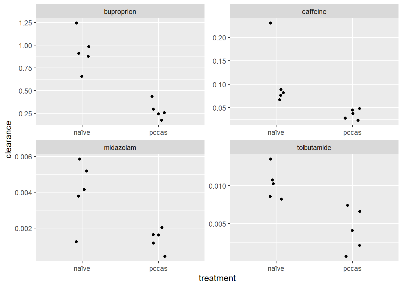
Figure 38.1: Drug clearance in a mouse model for malaria.
Print the linear model results to view the effect sizes as regression coefficients:
mod##
## Call:
## lm(formula = cbind(caffeine, tolbutamide, buproprion, midazolam) ~
## treatment, data = pkdata)
##
## Coefficients:
## caffeine tolbutamide buproprion midazolam
## (Intercept) 0.109098 0.010273 0.934385 0.004038
## treatmentpccas -0.072693 -0.006087 -0.654121 -0.002661Considering the graph above it should be clear what the intercept values represent. They are the means for the naive treatment groups. The ‘treatmentpccas’ values are the differences between the naive and pccas group means. Their values are equivalent to the slopes of the red lines in the graph. In other words, the ‘treatmentpccas’ values are the means of the pccas groups subtracted from the means of the naive groups.
Intercept and treatmentpccas correspond respectively to the general linear model parameters \(\beta_0\) and \(\beta_1\).
Another way to think about this is the intercept (\(\beta_0\)) is an estimate for the value of the dependent variable when the independent variable is without any effect, or \(X=0\). In this example, if pccas has no influence on metabolism, then drug clearance is simply \(Y= \beta_0\)
In regression the intercept can cause confusion. In part, this happens because R operates alphanumerically by default. It will always subtract the second group from the first. Scientifically, we want the pccas means to be subtracted from naive….because our hypothesis is that malaria will lower clearance. Fortunately, n comes before p in the alphabet, so the group means for p will be subtracted from group means for n and this happens automagically. For simplicity, it is always a good idea to name your variables with this default alphanumeric behavior in mind.
38.6.3.2 MANOVA post hoc
In this the data passes and omnibus MANOVA. It tells us that somewhere among the four dependent variables there are differences between the naive and pccas group means. The question is which ones?
As a follow on procedure we want to know which of the downward slopes are truly negative, and which are no different than zero.
We answer that in the summary of the linear model. There is a lot of information here, but two things are most important. First, the estimate values for the treatmentpccas term. These are differences in group means between naive and pccas. Second, statistics and p-values associated with the ‘treatmentpccas’ effect. These are a one-sample t-test.
These each ask, “Is the Estimate value, given its standard error, equal to zero?” For example, the estimate for caffeine is -0.07269, which is the slope of the red line above. The t-statistic value is -2.344 and it has a p-value just under 0.05.
We’re usually not interested in the information on the intercept term or the statistical test for it. It is the group mean for the control condition, in this case, demonstrating the background level of clearance. Whether that differs from zero not important to know.
tidy(mod)## # A tibble: 8 x 6
## response term estimate std.error statistic p.value
## <chr> <chr> <dbl> <dbl> <dbl> <dbl>
## 1 caffeine (Intercept) 0.109 0.0219 4.97 0.00109
## 2 caffeine treatmentpccas -0.0727 0.0310 -2.34 0.0471
## 3 tolbutamide (Intercept) 0.0103 0.00112 9.16 0.0000163
## 4 tolbutamide treatmentpccas -0.00609 0.00159 -3.84 0.00497
## 5 buproprion (Intercept) 0.934 0.0738 12.7 0.00000142
## 6 buproprion treatmentpccas -0.654 0.104 -6.27 0.000241
## 7 midazolam (Intercept) 0.00404 0.000592 6.82 0.000135
## 8 midazolam treatmentpccas -0.00266 0.000837 -3.18 0.0131Therefore to make the p-value adjustment we should only be interested in the estimates for the ‘treatmentpccas’ terms. We shouldn’t waste precious alpha on the intercept values.
Here’s how we do that:
tidy(mod) %>%
  select(response, estimate, p.value) %>%
  filter(row_number() %% 2 == 0) %>%
  mutate(p.value_adjusted=p.adjust(p.value,
                                   method="bonferroni"))
## # A tibble: 4 x 4
## response estimate p.value p.value_adjusted
## <chr> <dbl> <dbl> <dbl>
## 1 caffeine -0.0727 0.0471 0.188
## 2 tolbutamide -0.00609 0.00497 0.0199
## 3 buproprion -0.654 0.000241 0.000964
## 4 midazolam -0.00266 0.0131 0.0522Given a family-wise type1 error threshold of 5%, we can conclude that PccAS infection changes tolbutamide and buproprion clearance relative to naive animals. There is no statistical difference for caffeine and midazolam clearance between PccAS-infected and naive animals.
It should be noted that this is a very conservative adjustment. In fact, were the Holm adjustment used instead all four drugs would have shown statistical differences.
38.6.3.3 Write up
The drug clearance experiment evaluates the effect of PccAS infection on the metabolism of caffeine, tolbutamide, buproprion and midazolam simultaneously in two treatment groups, naive and PccAS-infected, with five independent replicates within each group. Clearance data were analyzed by a multiple linear model using MANOVA as an omnibus test (Pillai test statistic = 0.905 with 1 df, F(4,5)=11.943, p=0.009). Posthoc analysis usig t-tests indicates PccAS the reductions in clearance relative to naive for tolbutamide (-0.006 clearance units) and buproprion (-0.654 clearance units) are statistically different than zero (Bonferroni adjusted p-values are 0.0199 and 0.0009, respectively).
38.7 Planning MANOVA experiments
Collecting several types of measurements from every replicate in one experiment is a lot of work. In these cases, front end statistical planning can really pay off.
We need to put some thought into choosing the dependent variables.
MANOVA doesn’t work well when too many dependent variables in the dataset are too highly correlated and all are pointing in the same general direction. For example, when several different mRNAs increase in the same way in response to a treatment. They will be statistically redundant, which can cause computational difficulties and the regression fails to converge to a solution. The only recovery from that is to add the variables back to a model one at a time until the offending variable is found. Which invariably causes the creepy bias feeling.
Besides, it seems wasteful to measure the same thing many different ways.
Therefore, omit some redundant variables. Be sure to offset positively correlated variables with negatively correlated variables in the dataset. Similarly, MANOVA uncorrelated dependent variables should be avoided.
Use pilot studies, other information, or intuition to understand relationships between the variables. How are they correlated? Once we have that we can calculate covariances?
38.7.1 MANOVA Monte Carlo Power Analysis
The Monte Carlo procedure is the same as for any other test: 1)Simulate a set of expected data. 2)Run an MANOVA analysis, defining and counting “hits.” 3)Repeat many times to get a long run performance average. 4)Change conditions (sample size, add/remove variables, remodel, etc) 5)Iterate through step 1 again.
38.7.1.1 Design an MVME
Let’s simulate a minimally viable MANOVA experiment (MVME) involving three dependent variables. For each there are a negative and positive control and a test group, for a total of 3 treatment groups.
For all three dependent variables we have decent pilot data for the negative and positive controls. We have a general idea of what we would consider minimally meaningful scientific responses for the test group.
One of our dependent variables represents a molecular measurement (ie, an mRNA), the second DV represents a biochemical measurement (ie, an enzyme activity), and the third DV represents a measurement at the organism level (ie, a behavior). We’ll make the organism measurement decrease with treatment so that it is negatively correlated with the other two.
We must assume each of these dependent variables in normally distributed, \(N(\mu, \sigma^2)\). We have a decent idea of the values of these parameters. We have a decent idea of how correlated they may be.
All three of the measurements are taken from each replicate. Replicates are randomized to receiving one and only one of the three treatment groups.
The model is essentially one-way completely randomized MANOVA; in other words, one factorial independent variable at three levels, with three dependent variables.
38.7.1.2 Simulate multivariate normal data
The rmvtnorm function in the mvtnorm package provides a nice way to simulate several vectors of correlated data simultaneously, the kind of data you’d expect to generate and then analyze with MANOVA.
But it takes a willingness to wrestle with effect size predictions, correlations, variances and covariances, and matrices to take full advantage.
rmvtnorm takes as arguments the expected means of each variable, and sigma, which is a covariance matrix.
First, estimate some expected means and then their standard deviations. Then simply square the latter to calculate variances.
To predict standard deviations, it is easiest to think in terms of coefficient of variation: What is the noise to signal for the measurement? What is the typical ratio of standard deviation to mean that you see for that variable? 10%, 20%, more, less?
For this example, we’re assuming homoscedasticity, which means that the variance is about the same no matter the treatment level. But when we know there will be heterscedasticity, we should code it in here.
| treat | param | molec | bioch | organ |
|---|---|---|---|---|
| neg | mean | 270 | 900 | 0 |
| neg | sd | 60 | 100 | 5 |
| neg | var | 3600 | 10000 | 25 |
| pos | mean | 400 | 300 | -20 |
| pos | sd | 60 | 100 | 5 |
| pos | var | 3600 | 10000 | 25 |
| test | mean | 350 | 450 | -10 |
| test | sd | 60 | 100 | 5 |
| test | var | 3600 | 10000 | 25 |
38.7.1.2.1 Building a covariance matrix
For the next step we estimate the correlation coefficients between the dependent variables. We predict the biochem measurements and the organ will be reduced by the positive control and test treatments. That means they will be negatively correlated with the molec variables, where the positive and test are predicted to increase the response.
Where do these correlation coefficients come from? They are estimates based upon pilot data. But they can be from some other source. Or they can be based upon scientific intuition. Estimating these coefficients is no different than estimating means, standard deviations and effect sizes. We use imagination and scientific judgment to make these predictions.
We pop them into a matrix here. We’ll need this in a matrix form to create our covariance matrix.
A <- matrix(c(1, -0.8, -0.3, -0.8, 1, 0.6, -0.3, 0.6, 1 ),
       ncol=3, byrow=F,
       dimnames=list(c("molec", "biochem", "organ"),
                     c("molec", "biochem", "organ")
                     )
       )
A
## molec biochem organ
## molec 1.0 -0.8 -0.3
## biochem -0.8 1.0 0.6
## organ -0.3 0.6 1.0Next we can build out a variance product matrix, using the variances estimated in the table above. The value in each cell in this matrix is the square root of the product of the corresponding variance estimates (\(\sqrt {var(Y_1)var(Y_2)}\). We do this for every combination of variances, which should yield a symmetrical matrix.
B <- matrix(c(3600,6000,300,6000,10000,500,300,500,25), ncol=3, byrow=F,
            dimnames=list(c("molec", "biochem", "organ"),
                     c("molec", "biochem", "organ")
                     ))
B
## molec biochem organ
## molec 3600 6000 300
## biochem 6000 10000 500
## organ 300 500 25Here’s why we’ve done this. The relationship between any two dependent variables, \(Y_1\) and \(Y_2\) is
\[cor(Y_1, Y_2) = \frac{cov(Y_1, Y_2)}{\sqrt {var(Y_1)var(Y_2)}}]\]
Therefore, the covariance matrix we want for the sigma argument in the rmvnorm function is calculated by multiplying the variance product matrix by the correlation matrix.
sigmas <- A*B
sigmas
## molec biochem organ
## molec 3600 -4800 -90
## biochem -4800 10000 300
## organ -90 300 25Since we assume homescedasticity we can use sigmas for each of the three treatment groups. Now it is just a matter of simulating the dataset with that one sigma and the means for each of the variables and groups.
n <- 5

negMeans <- c(270, 900, 0)
posMeans <- c(400, 300, -20)
testMeans <- c(350, 450, -10)


neg <- rmvnorm(n,mean=negMeans, sigma=sigmas)
pos <- rmvnorm(n,mean=posMeans, sigma=sigmas)
test <- rmvnorm(n,mean=testMeans, sigma=sigmas)

outMat <- rbind(neg, pos, test)
Parenthetically, if we are expecting heteroscedasticity, we would need to calculate a different sigma for each of the groups.
Pop it into a data frame and summarise by groups to see how well the simulation meets our plans. Keep in mind this is a small random sample. Increase the sample size, \(n\), to get a more accurate picture.
sim <- data.frame(treatment=c(rep("neg_ctrl", n),
                          rep("pos_ctrl", n),
                          rep("test", n)
                          ),
              molec = outMat[ , 1],
              bioch = outMat[ , 2],
              organ = outMat[ , 3]
              )
sim %>% group_by(treatment) %>% summarise(meanMol=mean(molec),
                                          sdMol=sd(molec),
                                          meanBio=mean(bioch),
                                          sdBio=sd(bioch),
                                          meanOrg=mean(organ),
                                          sdOrg=sd(organ))
## # A tibble: 3 x 7
## treatment meanMol sdMol meanBio sdBio meanOrg sdOrg
## <chr> <dbl> <dbl> <dbl> <dbl> <dbl> <dbl>
## 1 neg_ctrl 316. 57.0 862. 181. 0.0251 9.50
## 2 pos_ctrl 418. 62.9 260. 109. -23.8 4.86
## 3 test 336. 75.8 439. 123. -11.3 6.75Now we run a the “sample” through a manova. We’re switching to base R’s manova here because it plays nicer than Manova with Monte Carlo
model <- lm(cbind(molec, bioch, organ) ~ treatment, data=sim)

man <- summary(manova(model))
man
## Df Pillai approx F num Df den Df Pr(>F)
## treatment 2 1.4379 9.3793 6 22 3.719e-05 ***
## Residuals 12
## ---
## Signif. codes: 0 '***' 0.001 '**' 0.01 '*' 0.05 '.' 0.1 ' ' 1Assuming this Manova test gives a positive response, we follow up with look post hoc at the key comparison, because we’d want to power up an experiment to ensure this one is detected.
Our scientific strategy is to assure the organ effect of the test group. Because one has nothig without the animal model, right?
So out of all the posthoc comparisons we could make, we’ll focus in on that.
tidy(model)## # A tibble: 9 x 6
## response term estimate std.error statistic p.value
## <chr> <chr> <dbl> <dbl> <dbl> <dbl>
## 1 molec (Intercept) 316. 29.4 10.8 0.000000161
## 2 molec treatmentpos_ctrl 101. 41.6 2.44 0.0313
## 3 molec treatmenttest 19.8 41.6 0.476 0.643
## 4 bioch (Intercept) 862. 63.1 13.7 0.0000000112
## 5 bioch treatmentpos_ctrl -603. 89.2 -6.76 0.0000203
## 6 bioch treatmenttest -423. 89.2 -4.75 0.000475
## 7 organ (Intercept) 0.0251 3.26 0.00768 0.994
## 8 organ treatmentpos_ctrl -23.8 4.61 -5.16 0.000237
## 9 organ treatmenttest -11.3 4.61 -2.46 0.0301The comparison in the 9th row is between the test and the negative control for the organ variable. The estimate means its value is -11.46 units less than the negative control. The unadjusted p-value for that difference is 0.0041. Assuming we’d also compare the test to negative controls for the other two variables, were’s how we can collect that p-value while adjusting it for multiple comparisons simultaneously.
The code below comes from finding a workable way to create test output so the parameter of interest is easy to grab. Unfortunately, output from the Manova function is more difficult to handle.
p.adjust(unname(as_vector(tidy(model)[9,6])),method="bonferroni", n=3)## [1] 0.0903492838.7.2 An MANOVA Monte Carlo Power function
The purpose of this function is to determine the sample size of suitable power for an MANOVA experiment.
This function pulls all of the above together into a single script. The input of this script is a putative sample size. The output is the power of the MANOVA, and the power of the most important posthoc comparison: that between the test group and negative control for the organ variable.
manpwr <- function(n){
#initializers
  #covariance matrix
  A <- matrix(c(1, -0.8, -0.3,
                -0.8, 1, 0.6,
                -0.3, 0.6, 1 ),
         ncol=3, byrow=F,
           dimnames=list(c("molec", "biochem", "organ"),
                     c("molec", "biochem", "organ")
                     ))

  B <- matrix(c(3600,6000,300,
                6000,10000,500,
                300,500,25),
            ncol=3, byrow=F,
            dimnames=list(c("molec", "biochem", "organ"),
                     c("molec", "biochem", "organ")
                     ))
  sigmas <- A*B
  #predicted means
  negMeans <- c(270, 900, 0)
  posMeans <- c(400, 300, -20)
  testMeans <- c(350, 450, -10)
  #misc function running variables
  manpval <- c()
  orgpval <- c()
  i <- 1
  ssims <- 100
  alpha <- 0.05
#Data simulator
 repeat {
    neg <- rmvnorm(n,mean=negMeans, sigma=sigmas)
    pos <- rmvnorm(n,mean=posMeans, sigma=sigmas)
    test <- rmvnorm(n,mean=testMeans, sigma=sigmas)
    outMat <- rbind(neg, pos, test)
    sim <- data.frame(treatment=c(rep("neg_ctrl", n),
                          rep("pos_ctrl", n),
                          rep("test", n)
                          ),
              molec = outMat[ , 1],
              bioch = outMat[ , 2],
              organ = outMat[ , 3]
              )
      model <- lm(cbind(molec, bioch, organ) ~
                    treatment, data=sim)

      manp <- summary(manova(model))$stat[11]
      manpval[i] <- manp
  #grab the p-value for the most important posthoc
      if (manp < alpha) {

          otp <- p.adjust(unname(
                as_vector(
                tidy(model)[9,6])),
                method="bonferroni", n=3)

          orgpval[i] <- otp
      }
      if (i==ssims) break
      i=i+1
  #prepare output
        manpwer <- length(which(manpval<alpha))/ssims
        orgpwr <- length(which(orgpval<alpha))/ssims
 }
   c(paste("manova power=", manpwer, sep=""),
     paste("posthoc power=", orgpwr, sep=""))
}
Here’s how to run manpwr. It’s a check to see the power for a sample size of 5 replicates per group.
The output is interesting. Although the MANOVA test is overpowered, the critical finding of interest is underpowered at this sample size. Repeat the function at higher values of n until the posthoc power is sufficient.
It is crucial to understand that powering up for the posthoc results can be so important.
manpwr(5)## [1] "manova power=0.99" "posthoc power=0.71"38.8 Summary
MANOVA is an option for statistical testing of multivariate experiments. The dependent variables are random normal The test is more senstive than other parametrics to violations of normality and homogeneity of variance. MANOVA tests whether independent variables affect an abstract combination of dependent variables. For most, use MANOVA as an omnibus test followed by post hoc comparisons of interest to control FWER. Care should be taken in selecting the dependent variables of interest.
#sessionInfo()