Chapter 10 Variability, Accuracy and Precision
“Your estimate can be imprecise or inaccurate or both and it is helpful to know why you may never know it.”
library(tidyverse)
library(ggformula)
Experimentalists draw random samples from a population we are interested in studying.
In statistical thinking, the population parameters that interest us are held to have true, fixed values. The random sample provides a way to estimate the value of these parameters.
The random sample will have variation. Even under the best of conditions, by random chance we will draw a sample that provides either a good or a not-so-good estimate of these fixed population parameters.
A major focus of statistics is about quantifying the uncertainty of how reliable are our parameter estimates. Which is very important because in turn that addresses the reliability of our understanding of the system that we are researching.
It is not possible to understand statistical analysis without wrapping our heads around the concepts related to data dispersion: variability, accuracy and precision. Together, these concepts comprise ways of thinking about and describing the uncertainty of data.
10.1 Data are messy
The reason data are messy is that sample data possess inherent variability. This means there is always some ‘error’ between the true values of the population parameters and their estimated values within the sample.
In running experiments on biological systems we think about two main contributors to this error. The first is biological variation between independent replicates.
The second source is so-called systematic error. These are related to our our processes, the techniques and equipment, the way we measure the sample.
These ways of thinking about different sources for variation will hopefully become more clear when we get to ANOVA and to regression.
10.2 Illustration of a model with error
As you recall from middle school, a straight line drawn between two variables is described by the linear model \(Y=\beta_0+\beta_1 X\). This model has two parameters, the parameter \(\beta_0\) represents the y-intercept while the parameter \(\beta_1\) represents the slope of the line. The independent variable (levels of which are controlled by the researcher) is \(X\). Thus, passing values of \(X\) into this model generates values for the response variable, \(Y\).
Here’s a simulation of response data from two linear related models, \(Y1\) and \(Y2\).
Reading the code, you notice that one of the models, \(Y1\) has no error term. So it is perfect, which is to say the values of \(Y1\) are perfectly predicted by the model’s intercept and slope parameters. A linear regression goes through every data point and the output of that regression yields the exact same parameter values that were input (a bit of a circular proof, if you will). The model perfectly fits its data.
The other model (\(Y2\)) has an error term tacked onto it. As a result it yields imperfect values even when given the exact same model parameters as for \(Y1\).
Applying a linear regression to \(Y2\) yields an imperfect fit…the line doesn’t go through all of the data points. Error is associated with the estimate (the gray shade), and the intercept and slope parameters estimated through linear regression differ somewhat from the parameter input values.
#intital model parameter values
b0 <- 0
b1 <- 5
X <- seq(1,10,1)
set.seed(8675309)
error <- rnorm(length(X), mean=0, sd=10)
#models
Y1 <- b0+b1*X
Y2 <- b0+b1*X + error
# long dataframe for easy plotting
df <- data.frame(X, Y1, Y2) %>%
  pivot_longer(cols=c(Y1, Y2),
               names_to="model",
               values_to="response")
#plotting function
ggplot(df, aes(X, response))+
  geom_point()+
  geom_smooth(aes(X, response), method=lm)+
  facet_grid(cols=vars(model))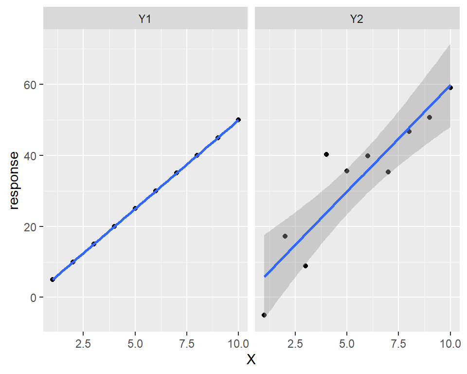
Figure 10.1: Models are perfect, data are not.
You can appreciate how the second model, with the random error term, is more real life.
What’s even more interesting is that every time you run the second model you’ll generate a completely different result (so long as you remove the set.seed() function. Copy and paste that code chunk into R and see for yourself. That error term is just a simulation of a random process. And that’s just how random processes behave!
(Play with that code if you don’t understand how it works. Run it on your machine. Change the initializers)
In real life we would only have the random values of the variable.
Unlike in this simulation, we wouldn’t know the true values of the parameters. In real life we sample, determine the model parameters, and test to see how well the imperfect data fit a perfect model with those parameters.
At this point in the course it’s not important to interpret what all of this error analysis means. The point I’m making right now, and that hopefully you’ll grow to appreciate, is that to a large extent, statistics is mostly about residual error analysis–measuring and accounting for the differences between perfect models and random data.
10.3 Variance: Quantifying variation by least squares
The two primary methods to quantify variation are termed “ordinary least squares” and “maximum likelihood estimation.” Mathematically they are distinct, and that difference is beyond the scope of this moment. What is important is that, in most cases, either method will arrive at roughly the same solution.
Ordinary least squares is the method used for quantifying variation for most of the statistics discussed in this course. The only exception is when we get to generalized linear models. So we’ll omit consideration of maximum likelihood estimation until then.
Ordinary least squares arises from the theoretical basis of variance and fully depends upon the following assertion:
A random variable, \(Y\), has an expected value equivalent to its mean, \(E(Y) = \mu\). It can be proven (by mathematicians…not me) that the variance of \(Y\) is the difference between it’s squared mean and its mean squared:
\[\begin{equation} Var(Y) = E(Y^2)-E(Y)^2 \tag{10.1} \end{equation}\]
In practice, imagine a sample of size \(n\) random independent replicates drawn from a population of the continuous random variable, \(Y\). The replicate sample values for \(Y\) are, \(y_i\), and thus \(y_1, y_2, ...y_n\).
The mean of these replicate values provides a point estimate for the mean of the sampled population, \(\mu\), and is
\[\begin{equation} \bar y = \frac{{\sum_{i=1}^n}y_i}{n} \tag{10.2} \end{equation}\]
The value by which each replicate within the sample varies from the mean is \(y_i-\bar y\). In jargon these are described alternately as a variate, or a deviate or as a residual. Each word represents the same thing.
A vector of sample replicates will have values that are smaller than and larger than the mean. Thus, some variate values are positive, while others are negative.
In a random sample of a normally distributed variable we would expect that the values for variates are roughly equally dispersed above and below a mean. Thus, if we were to sum up the deviates (or variates or residuals) we’d expect that that sum’s value to approach zero.
\[\begin{equation} E(\sum_{i=1}^n(yi-\bar y))=0 \tag{10.3} \end{equation}\]
By squaring the deviates, negative values of the deviates are removed, providing a parameter that paves the way to more capably describe the variation within the sample than can the sum of the deviates. This parameter is called the “sum of squares” or SS:
\[\begin{equation} SS=\sum_{i=1}^n(yi-\bar y)^2 \tag{10.4} \end{equation}\]
10.3.1 Definition of variance
A sample’s variance is the sum of the squared deviates divided by the sample degrees of freedom3, \(df=n-1\).
\[\begin{equation} s^2=\frac{\sum_{i=1}^n(yi-\bar y)^2}{n-1} \tag{10.5} \end{equation}\]
A sample’s variance, \(s^2\) is used as an estimate of the variance of the sampled population, \(\sigma^2\), in the same way \(y_bar\) estimates the population mean \(\mu\).
Since it is derived through division using a number that approximates sample size you can think of variance as an approximate average of \(SS\). Therefore, a synonym for variance is “mean square,” a jargon much used in ANOVA.
The reason \(s^2\) is arrived at through dividing by degrees of freedom, \(n-1\), rather than by \(n\) is because doing so produces a better estimate of the population variance, \(\sigma^2\). Mathematical proofs of that assertion can be found all over the internet.
Variance is a hard parameter to wrap the brain around. It describes the variability within a dataset, but geometrically: The units of \(s^2\) are squared. For example, if your response variable is measured by the \(gram\) mass of objects, then the variance units are in \(grams^2\).
That’s weird. Why do we do this?
The tl;dr answer is it is easier to detect differences when they are squared.
Later in the course, we’ll discuss statistical testing using analysis of variance (ANOVA) procedures. The fundamental idea of ANOVA is to test for group effects by “partitioning the error.” That’s actually done with \(SS\)…the squared variable. When a factor causes some effect, the \(SS\) associated with that factor get larger…by the square of the variation.
Statistical testing is then done on the variance in groups, which in ANOVA jargon is called the “mean square,” or \(MS\). \(MS\) is just another way for saying average variance.
10.4 Standard deviation
The sample standard deviation solves the problem of working with an unintuitive squared parameters. The standard deviation is a more pragmatic descriptive statistic than is variance.
The standard deviation is the square root of the sample variance:
\[\begin{equation} sd=\sqrt{\frac{\sum_{i=1}^n(y_i-\bar y)^2}{n-1}} \tag{10.6} \end{equation}\]
Poof! The weird squared value for the varible is gone. No more need to think about blood glucose in squared units of mg/dl.
10.4.1 What does the standard deviation tell us
The sample standard deviation is two things at once. It is
- a statistical parameter that conveys the variability within the sample.
- a point estimate of the variability within the population that was sampled.
There aren’t many factoids in statistics worth committing to memory, but the one that follows is:
A bit over two thirds of the values for a normally-distributed variable will lie between one standard deviation below and above the mean of that variable.
To “get” statistics it will be very important to get an intuitive feel for the standard deviation. I think the best way to understand it is to run R scripts that explore its properties.
Here’s one way to calculate the “two-thirds” rule using R’s pnorm function, the cumulative normal distribution function:
pnorm(-1, lower.tail = T) #Calculates the AUC below a zscore of -1.## [1] 0.1586553pnorm(1, lower.tail = F) #Calculates the AUC above a zscore of 1## [1] 0.15865531-pnorm(-1)-pnorm(1, lower.tail = F) #The middle range## [1] 0.6826895Explore: Use pnorm to calculate the AUC between z scores of -2 and 2, visualizing the outcome.
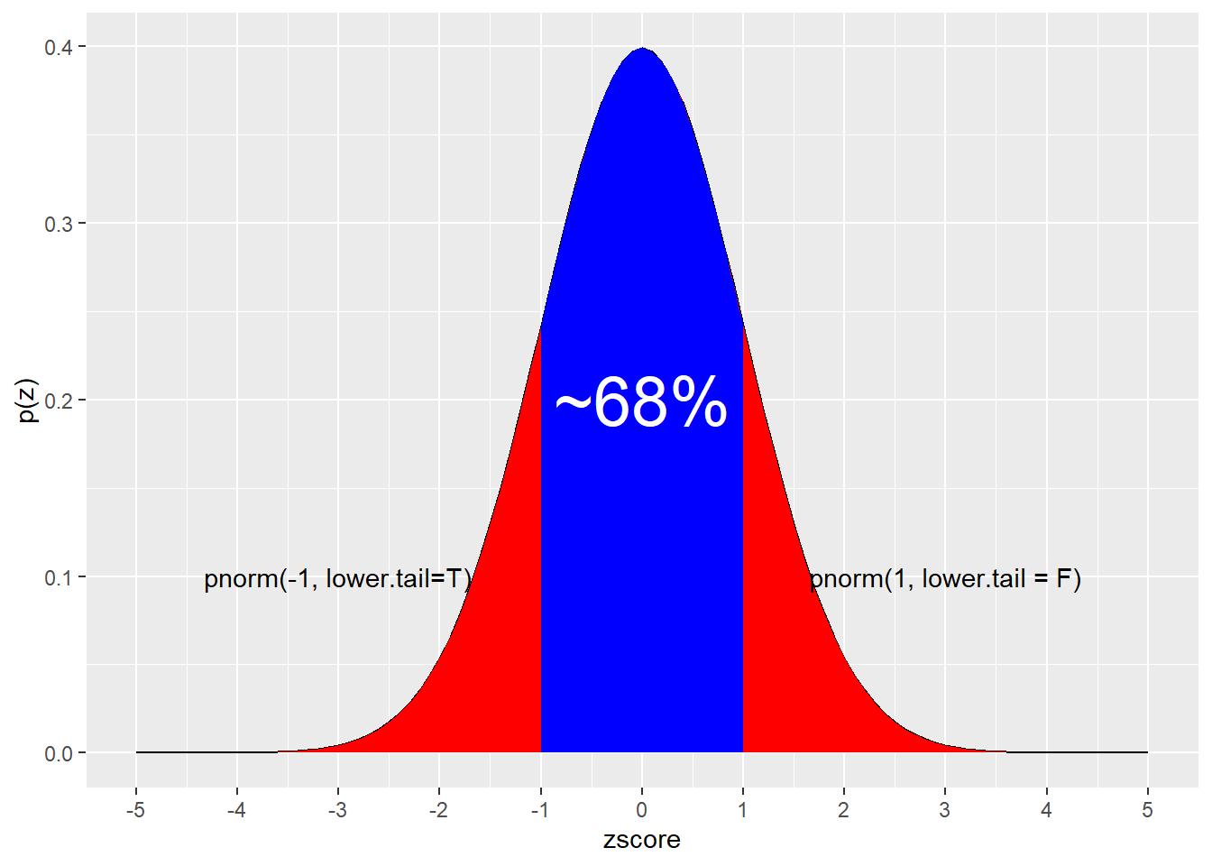
Figure 10.2: About 68% of the values for a normally distributed variable are within +/- one standard deviation from the mean.
No matter the scale for the variable, the relative proportion of values within 1 standard deviation for normally distributed variables will always behave this way. Here’s the distribution of serum glucose concentration values, where the average is 100 mg/dl and the standard deviation is 10 mg/dl:
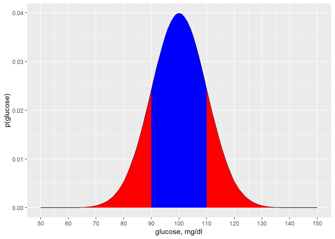
Figure 10.3: Modeling the distribution of a blood glucose variable.
10.4.2 Ways of describing sample variability
- Just show all of the data as scatter plots! Don’t hide the variability in bar plots with “error bars.”
- When using bar plots with error bars, always show SD.
- Violin plots are pretty ways to illustrate the spread and density of variation graphically.
- The coefficient of variation, \(cv=\frac{sd}{mean}\), is a dimensionless index that describes the noise-to-signal ratio.
- Percentiles and ranges. In particular, the interquartile range. This is usually reserved for non-normal data, particularly discrete data.
The SEM does not describe sample variability.
10.5 Precision and Accuracy
Even with well-behaved subjects, state-of-the-art equipment, and the best of technique and intentions, samples can yield wildly inaccurate estimates, even while measuring something precisely.
My favorite illustration of this is how estimates for the masses of subatomic particles have evolved over time. We can assume that the real masses of these particles have remained constant. Yet, note all of the quantum jumps, pun intended, in their estimated values.
What seems very accurate today could prove to be wildly inaccurate tomorrow. In particular, just because something is measured precisely doesn’t mean it is accurate.
10.6 Standard error
This will sound counter-intuitive, but we can actually know how precise our estimate of some parameter is without knowing the true value. That’s because precision is the repeatability of a measurement, and it is possible to repeat something very, very reliably but inaccurately.
The standard error is the statistical parameter used to express sample precision. Standard error is calculated from standard deviation and the sample size
\begin(equation) SE = \tag{10.7} \end(equation)
Thus, the SE is not something that estimates a fixed parameter of the sampled population. Since it reduces as sample size increases, it provides information only about the sample.
10.6.1 What exactly does the standard error represent?
The central limit theorem predicts a few important things:
- A distribution of many sample means will be normally distributed, even if a non-normal distribution is sampled.
- A distribution of sample means will have less dispersion with larger sample sizes.
- If a sample population has a mean \(\mu\) and standard deviation \(\sigma\), the distribution of sample means of sample size \(n\) drawn from that population will have a mean \(\mu\) and standard deviation \(\frac{\sigma}{\sqrt n}\).
Therefore, the standard error for a mean is the standard deviation of a theoretical population of sample means.
These features are illustrated below, as a prelude to further defining standard error.
The first graph showing a big boring black box. It simply plots out a uniform distribution of the random variable \(Y\) ranging in values from 0 to 1, using the duniffunction. It just means that any value, \(y\), plucked from that distribution is as equally likely as all other values. We’ll sample repeatedly from this distribution and show that the means of those samples are normally distributed.
ggplot(
  data.frame(
    x=seq(0, 1, 0.01)),
  aes(x))+
  stat_function(
    fun=dunif,
    args=list(min=0, max=1),
    xlim=c(0, 1),
    geom="area",
    fill="black")+
  labs(y="p(y)", x="Y")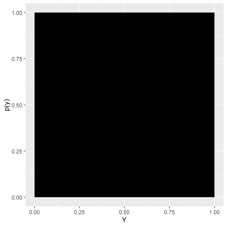
Figure 10.4: A variable having a uniform distribution
The probability of sampling any single \(y_i\) value is equivalent to that for all other \(y_i\) values. Uniform distributions arise from time-to-time. For example, important actually, the distribution of p-values derived from true null hypothesis tests is uniform.
As you might imagine, the mean of this particular uniform distribution is 0.5 (because it is halfway between the value limits 0 and 1). Probably less obvious is the standard deviation for a uniform distribution with limits \(a\) and \(b\) is \(\frac{b-a}{\sqrt{12}}\). So the standard deviation for this particular uniform distribution \(\sigma\) = 0.2887.
Just so you trust me, these two assertions pass the following simulation test:
mean(runif(n=100000, min=0, max=1))## [1] 0.498262sd(runif(n=100000, min=0, max=1))## [1] 0.2886213The next graph illustrates the behavior of the central limit theorem.
In the following a little custom function, called meanMaker, random samples are taken from this uniform distribution many times.
The script generates either 1000 means of very small random samples (n=3) or 1000 means from somewhat larger random samples (n=30).
Those two sets of means are then plotted.
Notice how the distributions of sample means are normally distributed, even though they comes from a uniform distribution! That validates the first prediction of the CLT, made above.
Note also that the distribution of means corresponding to the larger sample sizes has much less dispersion than that for the smaller sample sizes. That validates the second CLT prediction made above.
meanMaker <- function(n){
 mean(runif(n))
}
small.sample <- replicate(1000, meanMaker(3))
large.sample <- replicate(1000, meanMaker(30))
ggplot(data.frame(small.sample, large.sample))+
  geom_histogram(aes(small.sample), fill="red")+
  geom_histogram(aes(large.sample), fill="blue", alpha=0.5 )+
  xlab("n=3 (red) or n=30 (blue")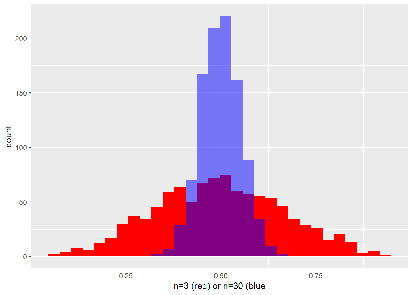
Figure 10.5: The central limit theorem in action, distributions of sample means of small (red) and large (blue) sample sizes.
As for the third point, the code below calculates a mean of all these means, and the SD of all these means, for each of the groups.
mean(small.sample)## [1] 0.4953052sd(small.sample)## [1] 0.1674984mean(large.sample)## [1] 0.4994673sd(large.sample)## [1] 0.05169953Irrespective of sample size, the mean of the means is a great estimator of the mean of the uniform distribution.
But passing the sample means into the sd function shows that neither provides a good estimate of the \(\sigma\) for the population sampled, which we know for a fact has a value of 0.2887.
Obviously, the standard deviation of a group of means is not an estimator of the population standard deviation. So what is it? The standard deviation of the distribution of sample means is what is known as the standard error of the mean.
This goes a long way to illustrate what the standard error of the mean of a sample, SEM, actually represents. It is an estimator of the theoretical standard deviation of the distribution of sample means,\(\sigma_{\bar y}\).
Now what are the implications of THAT?
There are a few.
First, SEM is not a measure of dispersion in a sample. It is a measure that describes the precision by which a mean has been estimated. The SEM for the large sample size group above is much lower than that for the small sample size group. Meaning, \(\mu\) is estimated more precisely by using large sample sizes. That should make intuitive sense.
Second, statistically naive researchers use SEM to illustrate dispersion in their data (eg, using SEM as “error bars”). Ugh. They do this because, invariably, the SEM will be lower than the SD. And they think that makes their results look cleaner.
But they should not do this, because SEM is not an estimator of \(\sigma\). Rather, SEM estimates \(\sigma_{\bar y}\). Those are two very different things.
When we do experiments we sample only once (with \(n\) independent replicates) and draw inferences about the population under study on that bases of that one sample.
We don’t have the luxury or resources to re-sample again and again, as we can in simulations. However, these simulations illustrate that, due to the central limit theorem, a long run of sampling is predictably well-behaved. This predictability is actually the foundation of statistical sampling methodology.
The SEM estimates a theoretical parameter (\(\sigma_{\bar y}\) that we would rarely, if ever, attempt to validate. Yet, on the basis of one sample it serves a purpose by providing an estimator of precision.
In a sense, the SEM provides an estimate for how well something is estimated.
10.6.2 “Should I use SD or SEM?”
The SEM does not illustrate variation. I suggest you use SEM if it is important to illustrate the precision by which something is measured. That’s usually only important for parameters that are physical constants. And the exact n should be coupled to every reported SEM. More often, your reader is better served by showing true dispersion. Use SD to summarize the variability in your data using SD.
10.7 Confidence intervals
Confidence intervals are among the most useful yet misunderstood statistics.
- They are calculated from a sample.
- They include the point estimate (eg, sample mean).
- They are a range of values of the parameter being estimated.
- They can be calculated for virtually any type of variable.
- There are many ways to calculate CIs
- They can be set at any confidence level the researcher prefers, 95%, 90%, 99%, 86.75309%
For example, assume the variable is blood glucose, in units of mg/dl, and the parameter we are interested in estimating is the mean blood glucose level in a population. The experiment involves taking a random sample of that population through \(n\) independent replicates, measuring the blood glucose level in each. The sample mean is calculated, along with a 95% confidence interval for that mean.
10.7.1 CI Definition
Let’s assume our experiment involves random sampling of a population to estimate its mean, and we are calculating the 95% confidence interval from that sample.
What does that 95% CI tell us?
Definition: We can be 95% confident confident that the population mean is within the interval.
In other words, for any given experiment there is a 1 in 20 chance the true value of the population mean is not within the 95% CI calculated from the sample.
Let me add that this is the beating heart of the frequentism, and it drives Bayesians apoplectic. The CI is a statistic that is calculated from the sample of one experiment…and yet its interpretation assumes an infinite number of repeats of that experiment would behave similarly. Something that we would never do.
More over, we have no idea what is the value for the true population mean and can never know it. Our sample may be wildly off. There is no assurance that repeated sampling will be any more reliable. We may be very wrong about our measuring method.
What does the 95% CI not mean?
- The 95% CI is not a probability.
We should neither say, “the probability of the point estimate is 95%” nor “the probability the true value lies within this range is 95%.”
The CI merely asserts a long run level of confidence in a range of values that might include the true parameter value. To have more or to have less confidence means that we would need to calculate some other interval, such as a 99% or 90% or 86.75309% interval. Changing the confidence level changes the range of the interval. Because our confidence in the sample changes!
10.7.2 Evaluating confidence intervals
The CI has duality as both and inferential and descriptive statistic. Standard errors and confidence intervals and test statistics and p-values are calculated from the same sample data. So there plenty of circular argument at play here.
The confidence interval serves as a statistical parameter used to express sample accuracy.
We use the variability within the sample to generate two related parameters, standard error and confidence intervals. If the former tells us about the precision of the point estimate (eg, the sample mean), let the latter speak to accuracy (eg, a range of sample means consistent with the sample that we can be confident of).
To be sure, this is conditioned on the experiment’s ability to detect a true point estimate. There are a lot of ways for the sample to be untrue. If the measurement machines and techniques are uncalibrated, or the sampled population is the wrong one, or there are uncontrolled confounder variables, or the experiment was underpowered, or the researcher picked and chose replicates to keep creating a biased sample, the sample may be wildly inaccurate.
Always realize the CI also reports the accuracy of point estimates that are wrong. Such wrong point estimates are something that can only be addressed scientifically, not statistically.
The confidence interval can be used inferentially, to make decisions on hypothesis tests
Assume three experiments, each by one of three different groups, are conducted to test whether a drug lowers blood glucose in diabetics. They all use a paired, before/after paradigm.
From each random independent replicate blood glucose is measured just before (B) and after (A) giving the drug. The estimated sample parameter is the mean difference between the before and after blood glucose values (a difference equal to \(B-A\) is computed within each replicate, the experiment tests whether that difference is reliable).
The null hypothesis is the mean difference is zero, or:
\[H_0:\beta - \alpha = 0\]
CI’s for the mean difference by the groups are listed:
- Group1: 95% CI: 57 to 25 mg/dl
- Group2: 95% CI: 34 to 2 mg/dl
- Group3: 95% CI: 40 to -5 mg/dl
Each group is 95% confident the true mean difference in blood glucose lies within their own calculated range.
The range of values in Group1 does not include the null value, zero. Using the CI alone, we can reject the null at a 95% confidence level. Further, given our scientific experitise in blood glucose, we also assert every value in that range is scientifically meaningful and may represent the true value.
The range of values in Group2 does not include the null value, zero. We can reject the null at a 95% confidence level. However, given our scientific expertise in blood glucose, we note the range includes low values that represent scientifically inconsequential effects. A change of 2 mg/dl may be “true” but is just not meaningful. Yet, it is in the range of possibilities. We should be extra suspicious of the reliability of the sample.
The range of values in Group3 does include the value of zero, which represents no mean difference. We are not prepared to reject the null at 95% confidence. We cannot conclude the drug has no effect. But the result is inconclusive.
10.7.3 CI Simulation tools
I’ve found simulation is by far the best way to gain an intuitive feel for how confidence intervals operate.
10.7.3.1 Evaluating one sample CI
The first random sampler is a script that generates a single random sample from a known distribution before calculating several sample parameters, including the confidence interval, which it plots as a pretty CI line over the distribution curve for the population that was sampled.
It’s particularly useful to illustrate the relationships between confidence intervals, sample sizes, standard deviations, confidence levels, and the sampled population.
When the confidence interval includees the mean of the population sampled, the confidence interval is accurate, and a blue-colored bar appears. When the confidence interval is not accurate, you get a red bar.
The confidence interval for a sample mean is calculated as follows:
\[CI=\bar x \pm t_{df(n-1)}\cdot\frac{sd}{\sqrt{n}}\]
#set.seed(8675309)
# change these initializers
n <- 3
pop.mean <- 100
pop.sd <- 25
sig.dig <- 2
conf.level <- 0.95
x <- c(seq(1, 200, 0.1))
# this draws a sample and calculate its descriptive stats
mysample <- rnorm(n, pop.mean, pop.sd)
mean <- round(mean(mysample), sig.dig)
sd <- round(sd(mysample), sig.dig)
sem <- round(sd/sqrt(n), sig.dig)
ll <- round(mean-qt((1+conf.level)/2,
                    n-1)*sem, sig.dig)
ul <- round(mean+qt((1+conf.level)/2,
                    n-1)*sem, sig.dig)
#print to console
print(c(round(mysample, sig.dig),
        paste(
          "mean=", mean, "sd=", sd,
          "sem=", sem, "CIll=", ll,
          "CIul=", ul)))
## [1] "79.48"
## [2] "170.74"
## [3] "84.11"
## [4] "mean= 111.45 sd= 51.4 sem= 29.68 CIll= -16.25 CIul= 239.15"# graph the sample confidence interval on the population
pretty <- ifelse(ll > pop.mean | ul < pop.mean, "red", "blue")
#graph (note: using ggformula package)
gf_line(dnorm(x, pop.mean, pop.sd)~x)%>%
gf_segment(0 + 0 ~ ll + ul,
size = 2,
color = pretty)%>%
gf_labs(subtitle =
paste(100*conf.level,
"% CI =",ll,
"to",ul))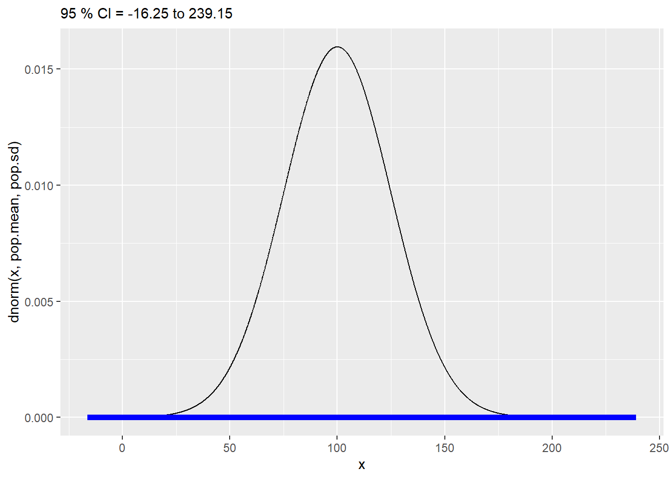
Figure 10.6: Confidence interval illustrator
10.7.3.2 Comparing two samples with CI
Here’s a second script that compares the confidence intervals of two means, from random samples of known distributions.
When two CI’s don’t overlap, they remain colored blue and green, and the two means they correspond to are unequal. It’s no different inferentially than test of a statistical difference for comparing two means and using p-values.
If the two CI’s overlap, one of them turns red. It’s a sign the two samples might not differ, since the 95% CI of one sample includes values in the 95% CI of the other. It’s also the same as a test of significance, for a null outcome.
Use this simulator to gain an intuitive understanding about how confidence intervals operate. Practice changing the sample size (n), the population means and standard deviations, and even the confidence level. Under what conditions are overlapping intervals diminished? What factors influence narrower intervals?
n <- 5
m <- 100
conf.level=0.95
t <- qt((1+ conf.level)/2, n-1)
pop.mean.A <- 125
pop.mean.B <- 200
pop.sd.A <- 25
pop.sd.B <- 25
x <- c(seq(1, 300, 0.1))
y <- seq(0.0005, m*0.0005, 0.0005)
#simulate
mydat.A <- replicate(
  m, rnorm(
    n, pop.mean.A, pop.sd.A
    )
  )
ldat.A <- apply(
  mydat.A,
  2,
  function(x) mean(x)-t*sd(x)/sqrt(n)
  )
udat.A <- apply(
  mydat.A,
  2,
  function(x) mean(x)+t*sd(x)/sqrt(n)
  )

mydat.B <- replicate(
  m, rnorm(
    n, pop.mean.B, pop.sd.B
    )
  )
ldat.B <- apply(
  mydat.B,
  2,
  function(x) mean(x)-t*sd(x)/sqrt(n)
  )
udat.B <- apply(
  mydat.B,
  2,
  function(x) mean(x)+t*sd(x)/sqrt(n)
  )

ci <- data.frame(
  y, ldat.A, udat.A, ldat.B, udat.B
  )

alt <- ifelse(
  udat.A >= ldat.B, "red", "blue"
  )

#plots made with ggformula package

gf_line(dnorm(
  x, pop.mean.A, pop.sd.A)~x,
  color = "dark green"
  )%>%

  gf_line(dnorm(
    x, pop.mean.B, pop.sd.B)~x,
    color = "blue"
    )%>%

  gf_segment(
    y+y ~ ldat.A + udat.A,
    data = ci,
    color = "dark green"
    )%>%

  gf_segment(
    y+y ~ ldat.B + udat.B,
    data = ci,
    color = alt
    )%>%
  gf_labs(
    y = "dnorm(x, pop.mean, sd.mean"
    )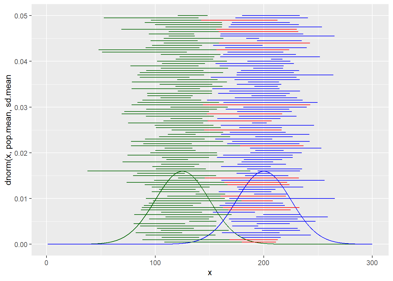
Figure 10.7: Comparing two samples using confidence intervals. Red-colored indicates the two CI overlap, meaning the two groups for that sample test out as no different.
10.8 Key take aways
Focus less on point estimates (eg, the mean of samples) and much more on the statistical parameters that give insight into variation (eg, SD, CI’s, range, and even SE)
- Variability is inherent in biological data. The two main sources are intrinsic biological variation–which has so many causes, and variability associated with our measurements and procedures.
- Statistics operates on the presumption that the values of parameters in the populations we sample are fixed. Residual error is unexplained deviation from those fixed values.
- About two-thirds of the values of a normally distributed variable will lay, symmetrically, within one standard deviation on either side of the variable’s mean.
- Variance expresses the variability within a sample, but geometrically, in squared units.
- The standard deviation, the square root of variance, estimates the variability of a sampled population.
- The standard error of the mean estimates the precision by which a sample mean estimates a population mean.
- The standard error of the mean grows smaller as sample size gets larger, by the square root of n.
- The standard error of the mean is the standard deviation of a theoretical distribution of sample means.
- A confidence interval estimates the accuracy by which a parameter, such as a mean, has been estimated.
- If the confidence intervals of two samples do not overlap, the sampled distributions likely differ.
- For a 95% CI for a mean, there is a 95% confidence the interval includes the true mean.
- A 99% CI will be wider than a 95% CI, given the same data. A 90% CI will be narrower.
- The best way to understand these various statistics of dispersion is to simulate and view the outcomes.
The sample mean is used to calculate SS; deriving that mean cost 1 degree of freedom. Given that mean, the values for all but one replicate are free to vary for the SS to be true. ↩︎