Chapter 37 ANOVA power using Monte Carlo

library(ez)
library(tidyverse)
library(viridis)

Monte Carlo simulation is a great tool for statistical design of experiments.

Monte Carlo forces us to do several things that, taken together, are characterize as good statistical hygiene.

• Explicitly define predictor variables and their levels
• Explicitly consider expected values and variation of the response variable
• Select scientifically meaningful groups to compare
• Consider which hypotheses is to be tested in advance
• Define a minimal scientifically meaningful effect size
• Establish a sample size a priori
• Establish the data munging and statistical analysis a priori
• Establish feasibility of the experiment a priori

If we want to do unbiased research (and we should) Monte Carlo simulation helps do exactly that. Design the experiment in advance. Analyze a simulation of the experiment, in advance. Figure out what we are going to do, in advance.

Then we go and conduct and analyze the experiment we designed.

The primary output of the Monte Carlo script below is experimental power at given sample sizes. We run the script primarily to know the number of independent replicates that are necessary to observe the effect size that we anticipate.

But conducting a Monte Carlo offers much more than just sample size.

An ability to ‘see’ experimental outcomes prior to running an experiment is the heartbeat of [turning predictions into strong testable hypotheses]. See Chapter 11.

Poking around with simulated data before running an experiment helps to critically evaluate our assumptions. This helps us see what might be missing before investing the time and expense in an experiment.

It also helps practice a statistical analysis. There is nothing unethical about p-hacking, harking and data snooping when playing with simulated data. All of tat helps design the analysis in a way that gives the best chance of observing the expected result!

Figuring that out before the real data set is in front of us helps avoid ethical gray areas after the real data set is in front of us.

37.1 Alternatives to Monte Carlo

Using R we can run the power.anova.testfunction in the base stats package or pwr.anova.test in the pwr package. To produce a sample size output, both of these require an entry for number of groups, type1 error and type2 error tolerance.

The former requires estimates for model (between) and residual (within) variance. These can be entered as relative values.

The latter requires an entry for Cohen’s \(f\). \[f=\sqrt{\frac{\eta^2}{1-\eta^2}}\] where \(\eta^2=\frac{SS_{model}}{SS_{total}}\) for a completely randomized factor, whereas for a related measures factor it is \(\eta_p^2=\frac{SS_{model}}{SS_{model}+SS_{residual}}\)

That’s great. But without a lot of experience these can be difficult values to estimate because they are not very intuitive.

37.2 What is Monte Carlo

As the name implies, Monte Carlo is based on random chance. Monte Carlo is a simulation tool to mimic random sampling.

In a single cycle of a Monte Carlo we simulate a random sample for an experiment, and run a statistical analysis to decide whether the experiment worked or not.

This is repeated many times. Hundreds or even thousands of times. What fraction of these repetes worked? That fraction is the experimental power. If the power is too low, we can adjust the experimental parameters and re-run. Or we can re-design the experiment entirely.

Once the Monte Carlo simulations yield an acceptable power, we have a sample size for conducting the real life experiment.

The process of creating a Monte Carlo script forces us to consider, explicitly, the variables in the experiment. What are their expected values? What effect size do we predict or think will be minimally scientifically significant? How many groups are in the experiment? Do these groups help us answer the question we really want answered? Should we add more groups or fewer groups?

Is the experiment under- or over-designed, or even feasible?

Is there a better way to answer the question?

Spending an hour or two going through this process in silico, optimizing and validating the experimental design, can save months of futile effort doing the wrong experiment in real life.

The first series of scripts below are for a one-way completely randomized ANOVA design. After that, a one-way related measures ANOVA Monte Carlo is shown. Their simulations differ in a couple of notable respects.

37.3 One-way completely randomized ANOVA Monte Carlo

The Outcome variable is random, continuous, and measured on an equal, or nearly equal interval, scale.

The experiment is comprised of \(k\ge3\) groups representing different levels of the Predictor variable.

The group variances are equivalent.

Every replicate (n) is independent of every other replicate.

37.3.1 Directions

1. Create initial values.
2. Visualize one random sample.
3. Run the Power Simulator
4. Change n and repeat until a suitable power is achieved.

37.3.2 Step 1: Create initial values

This is where we predict results.

I like making these Monte Carlo projects using a stand-alone initializer section. The whole point of the script is to play around with different initial parameters! Using an initializer section means we change these in only one place.

Here’s the logic:

First, provide an estimate for the expected mean of the outcome variable under basal conditions. Next, predict the fold-to-basal effect sizes for the positive control and also the treatment we’re planning to test. Next, estimate the value of the standard deviation of the Outcome variable. Finally, select the number of replicates per group (n per k) that we might run.

b = 100 #expected basal outcome value
a = 1.5 #expected fold-to-basal effect of our positive control
f = 1.25 #minimal scientifically relevant fold-to-basal effect of our treatment
sd = 25 #expected standard deviation of Outcome variable
n = 3 # number of independent replicates per group
sims = 100 #number of Monte Carlo simulations to run. 

37.3.3 Step 2: Visualize one random sample

This produces one graph illustrating an example of the type of random samples we’re generating in the Monte Carlo. No two samples will be the same, because they’re each random! So this figure will change every time it is run, even with the same initial parameter values. And because variances can differ a lot between groups with small sample sizes (n<35).

# Use this script to simulate our custom sample.
CRdataMaker <- function(n, b, a, f, sd) { 
  a1 <- rnorm(n, b, sd) #basal or negative ctrl
  a2 <- rnorm(n, (b*a), sd) #positive control or some other treatment
  a3 <- rnorm(n, (b*f), sd) #treatment effect
    Outcome <- c(a1, a2, a3)
    Predictor <- as.factor(c(rep(c("a1", "a2", "a3"), each = n)))
    ID <- as.factor(c(1:length(Predictor)))
    df <-data.frame(ID, Predictor, Outcome)
    }
dat <- CRdataMaker(n,b,a,f,sd)
ggplot(dat, aes(Predictor, Outcome))+
  geom_jitter(width=0.1,size = 4, alpha=0.5)

## Warning in (function (kind = NULL, normal.kind = NULL, sample.kind = NULL) :
## non-uniform 'Rounding' sampler used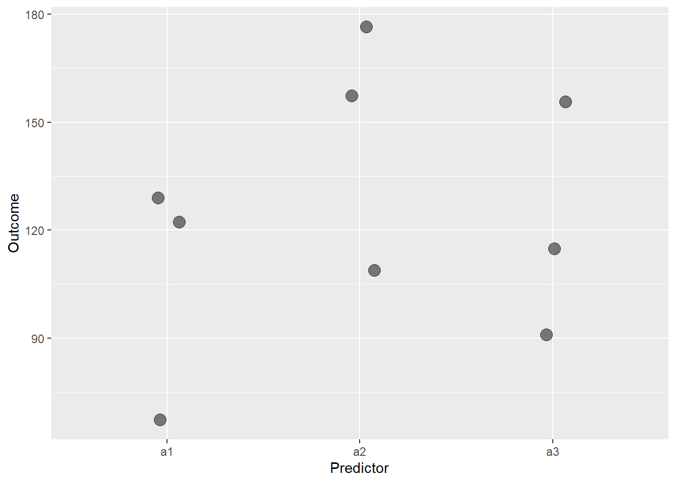

Figure 37.1: Representative simulated random sample for a one-way completely randomized ANOVA.

Is that what we expect to see? Should there be more variation? Is the effect size larger or smaller than what we anticipate? Should we add more or fewer groups?

Edit the code in the initializer to make it as real life as possible.

37.3.4 Step 3: Run The Power Simulator

Returns power (as a percentage value) for an experiment conducted given the values of the initializer variables.

Change n in the initializer above to see what it takes to get 80% or better power.

Carefully look at this code. It creates an ezANOVA output object, and then goes in to collect the p-value of the ANOVA F test from the ANOVA table.

pval <- replicate(
  sims, {
    sample.df <- CRdataMaker(n, b, a, f, sd)
    sim.ezaov <- ezANOVA(
            data = sample.df, 
            wid = ID,
            dv = Outcome,
            between = Predictor,
            type = 2
            )
  pval <- sim.ezaov$ANOVA[1,5]
    }
  )
pwr.pct <- sum(pval<0.05)/sims*100
paste(pwr.pct, sep="", "% power. Change 'n' in our initializer for higher or lower power.")

## [1] "37% power. Change 'n' in our initializer for higher or lower power."

ggplot(data.frame(pval))+
  geom_histogram(aes(pval), color="#d28e00")+
  labs(x="p-value")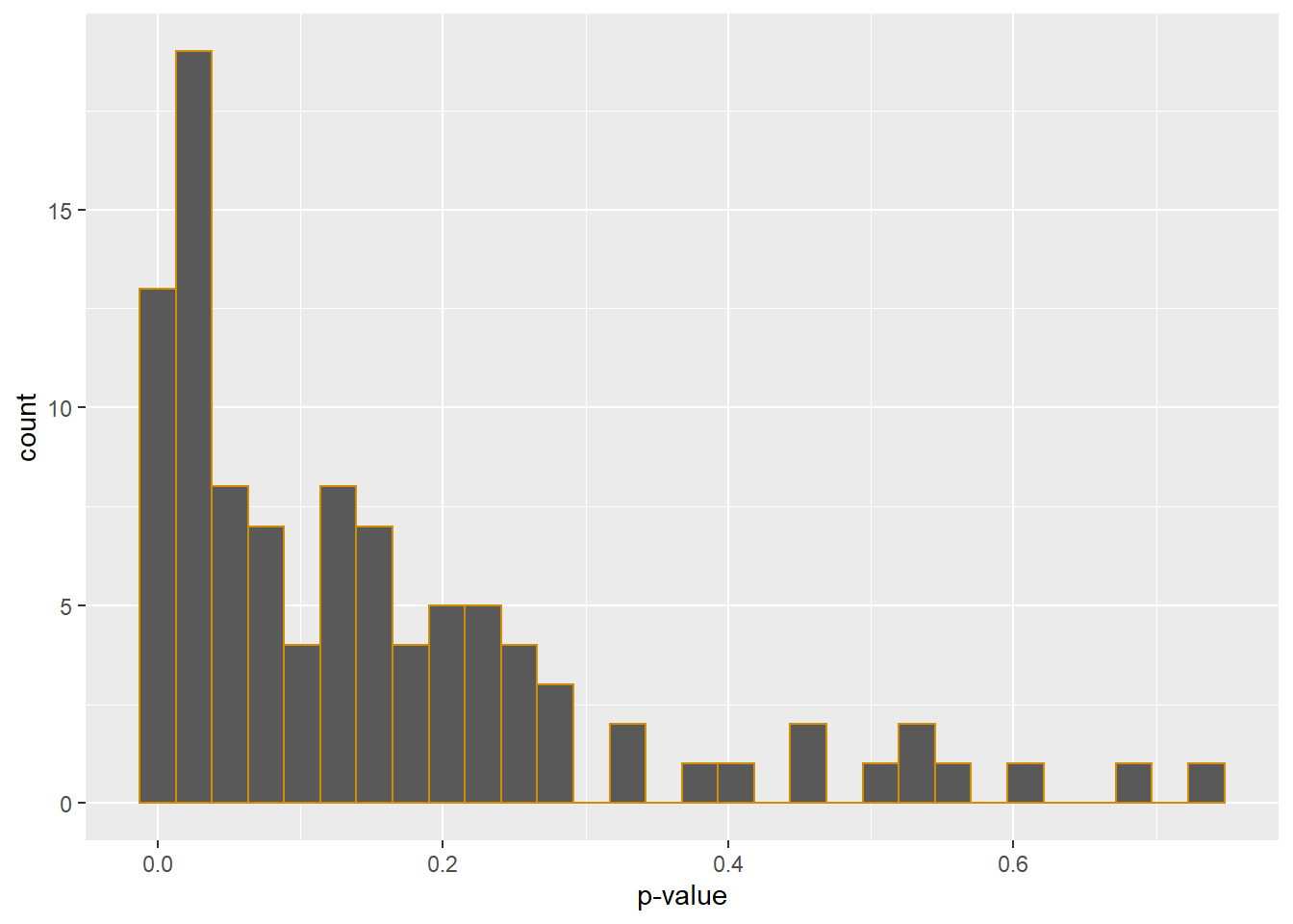

Figure 37.2: P-value distribution for a one-way repeated measures ANOVA Monte Carlo.

This could be modified. For example, here it collects the post hoc comparison between the test group and the negative control. Why is the power so much lower for this comparison compared to the power for a positive ANOVA?

pval <- replicate(
  sims, {
    sample.df <- CRdataMaker(n, b, a, f, sd)
    pval <- pairwise.t.test(sample.df$Outcome, sample.df$Predictor)$p.value[2,1]
    }
  )
pwr.pct <- sum(pval<0.05)/sims*100
paste(pwr.pct, sep="", "% power. Change 'n' in our initializer for higher or lower power.")

## [1] "14% power. Change 'n' in our initializer for higher or lower power."

ggplot(data.frame(pval))+
  geom_histogram(aes(pval), color="#d28e00")+
  labs(x="p-value")

## `stat_bin()` using `bins = 30`. Pick better value with `binwidth`.

Figure 37.3: P-value distribution for a one-way completely randomized ANOVA Monte Carlo

37.3.5 Step 4: Optimize for suitable power

The initializer is preconfigured with a fairly crappy experiment, comprised of a low sample size and not particularly strong effect size. As we can see the power calculation is also pretty crappy. About a third of experiments run in this way are likely to yield positive results.

Iteratively increase n until we get a more defensible level of power. Or maybe we need to change the estimates for the effect sizes?

37.3.6 Notes And Considerations

At k = 3 this is the minimal ANOVA design (any fewer groups and we’d just do a t test). This k = 3 experiment represents a minimal defensible scientific experiment: It has a negative control, a positive control, and the experimental.

The example above is also a simple one-way ANOVA completely randomized. Modifying the code to two-way and even three-way ANOVA designs is fairly trivial. we just add more groups. For example, if we have a second factor, Factor B and two levels, estimate the b1 and b2 results in much the same way the a1, a2 and a3 results are estimated.

we’ll need to adjust how the data frame is created, adding a column for the levels of Factor B.

Further modification will likely be necessary to collect a run of p-values for a specific group comparison. we may wish to grab the p-value for the interaction F test. Alternately, we may wish to go for a key posthoc comparison.

37.4 One-way related measures ANOVA Monte Carlo

The script below is a modification of that above, so that one way related measures ANOVA experiments can be simulated. There are two key differences. The first is adding a correlation coefficient to the initializer. The second is in the arguments for the ANOVA test function (from classifying the predictor variable from between to within).

The intrinsically-linked measurements that are a hallmark of related measures ANOVA tend to have high inherent correlation. This correlation should be taken into account when simulating related/repeated measure ANOVA experiments.

37.5 Directions

1. Create initial values.
2. Visualize one random sample.
3. Run the Power Simulator
4. Change n and repeat until a suitable power is achieved.

37.5.1 Step 1: Initial values

Here’s our initializers. Note the added terms r and k. Read Chapter 27 to understand what they represent and how we can estimate them for our system.

b <-  100 #expected basal outcome value
a <-  1.25 #expected fold-to-basal effect of our positive control
f <-  1.4 #minimal scientifically relevant fold-to-basal effect of our treatment
sd <-  25 #expected standard deviation of Outcome variable
n <-  3 # number of independent replicates per group
r <- 0.9 #correlation between groups of outcome values across replicates
k <- sqrt(1-r^2) #a conversion factor
sims = 100 #number of Monte Carlo simulations to run. Keep it low to start.

37.5.2 Step 2: Visualize one sample

Make sure we understand how the a2 and a3 variables were each correlated to the a1 variable. Let’s call a1 the pivot variable. When simulating correlated values, our pivot variable should be the lowest expected outcome value in the data set.

# Use this script to simulate a sample.
RMdataMaker <- function(n, b, a, f, sd, r, k) { 
  a1 <- rnorm(n, b, sd) #basal or negative ctrl
  a2 <- a1*r+k*rnorm(n, (b*a), sd) #positive control or some other treatment
  a3 <- a1*r+k*rnorm(n, (b*f), sd) #treatment effect
    Outcome <- c(a1, a2, a3)
    Predictor <- as.factor(c(rep(c("a1", "a2", "a3"), each = n)))
    ID <- rep(as.factor(c(1:n)))
    df <-data.frame(ID, Predictor, Outcome)
    }
dat <- RMdataMaker(n,b,a,f,sd,r,k)
ggplot(dat, 
       aes(Predictor, Outcome, color=ID, group=ID)
       )+ 
  geom_line()+
  geom_point(size = 4, shape=5)+
  scale_color_viridis(discrete=T)+
  theme_classic()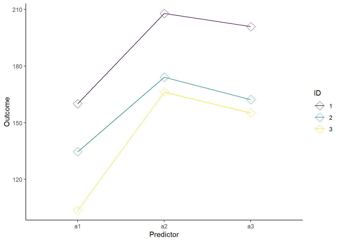

Figure 37.4: Representative simulated results for a one-way related measures ANOVA.

37.5.3 Step 3: Run the power simulator

Now we can simulate a long run of random samples like above, capturing how many of them yielded a positive result!

pval <- replicate(
  sims, {
    sample.df <- RMdataMaker(n, b, a, f, sd, r, k)
    sim.ezaov <- ezANOVA(
            data = sample.df, 
            wid = ID,
            dv = Outcome,
            within = Predictor,
            type = 2
            )
  pval <- sim.ezaov$ANOVA[1,5]
    }
  )
pwr.pct <- sum(pval<0.05)/sims*100
paste(pwr.pct, sep="", "% power. Change 'n' in the initializer for higher or lower power.")

## [1] "99% power. Change 'n' in the initializer for higher or lower power."

ggplot(data.frame(pval))+
  geom_histogram(aes(pval), color="#d28e00")+
  labs(x="p-value", title="p-value distribution")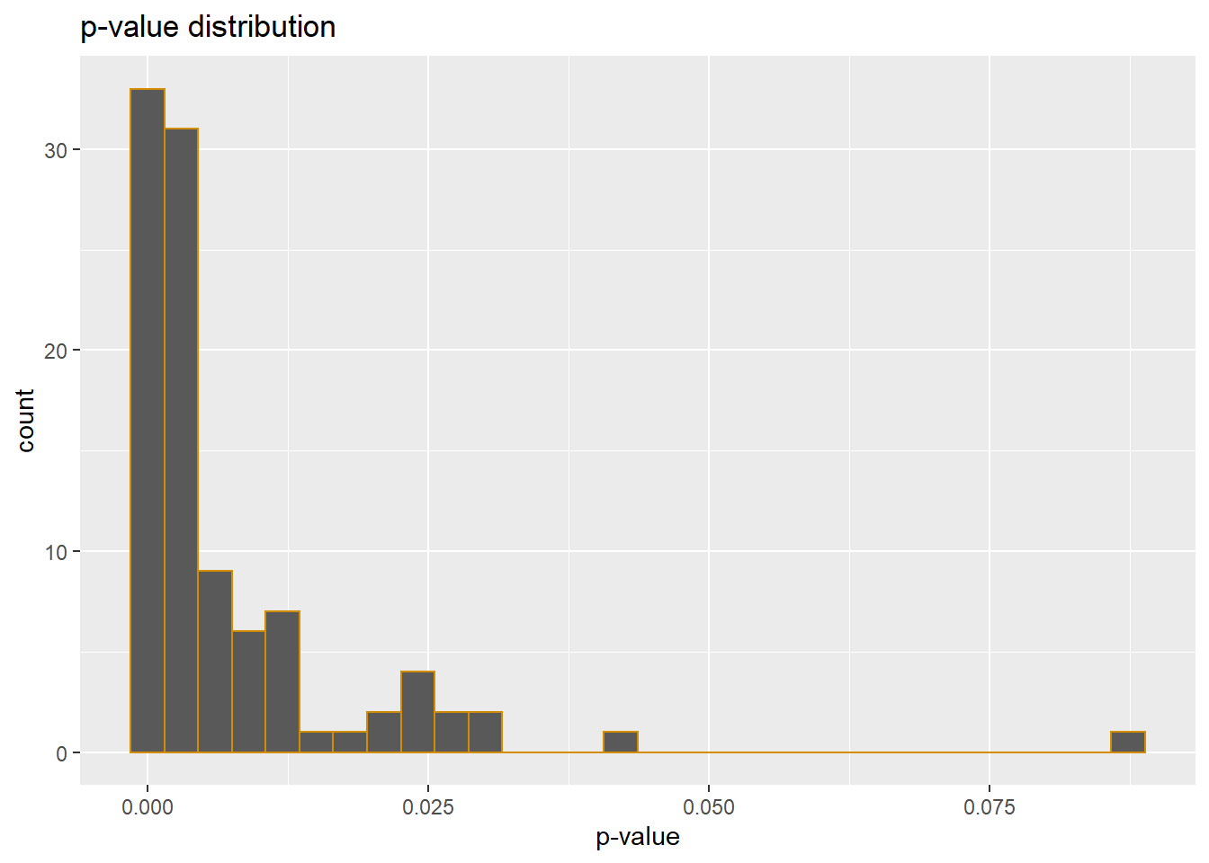

Figure 37.5: P-value distribution for a one-way repeated measures ANOVA Monte Carlo

37.5.4 Step 4: Should anything be changed?

The experiment simulated above has an n=3 and power of 99%! Notice how it has the same estimated group values as for the completely randomized simulation above, which yields only ~30% power.

That’s the efficiency of related measures! But we might want to experiment with changing correlation coefficient and sample size to see how the results are affected.

As for the completely randomized scripts, this one can be easily extended by adding more groups, or even more factors. we’ll need to make changes in all three script stages to customize our needs.