Chapter 28 Introduction to ANOVA

library(tidyverse)
library(RColorBrewer)

We typically turn to the analysis of variance (ANOVA) models when our experiments involve 3 or more groups and where the dependent variable values are continuous measures on an equal interval scale.

ANOVA experimental designs measure simultaneously the effects of multiple levels of a factor and/or multiple factors on these measurements.

Evaluating several effects simultaneously means that ANOVA designs can be very efficient. ANOVA is also quite versatile in terms of the number of factors involved and the number of measures that are taken from a given independent replicate.

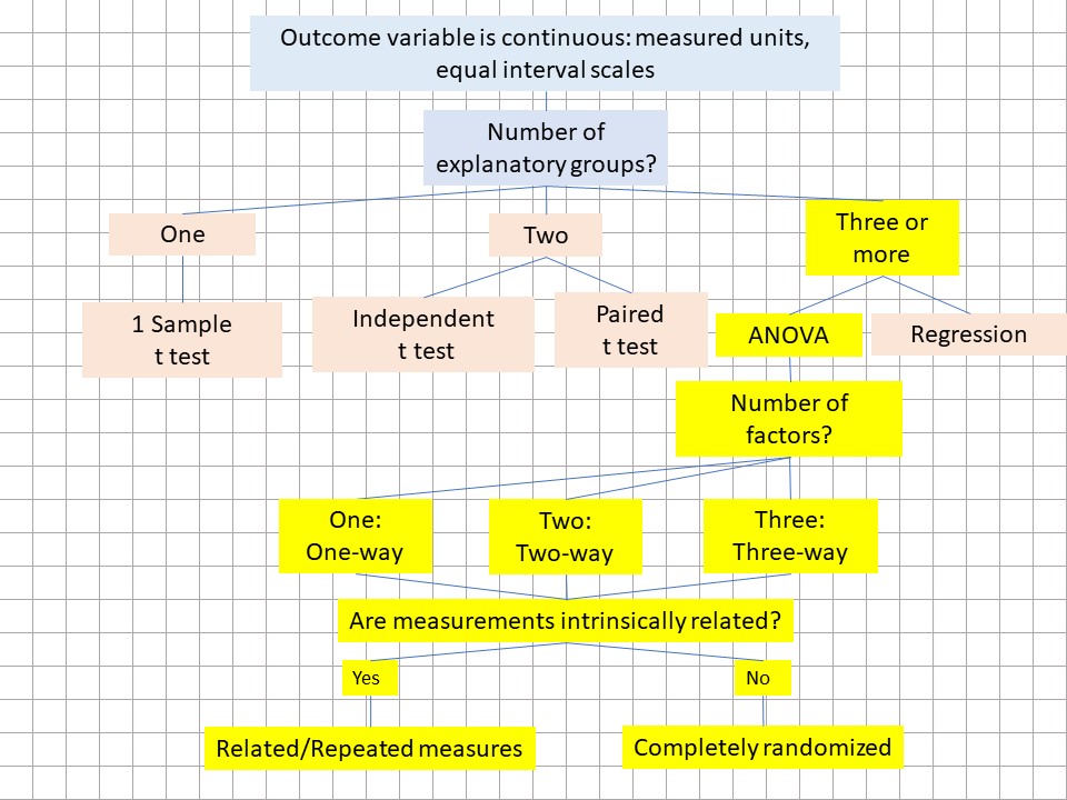
Figure 28.1: The ANOVA heuristic. ANOVA models involve 3 or more groups and the type of ANOVA depends upon the number of factors and whether related measures are involved.

ANOVA is also univariate, in so far as the analysis involves only a single dependent variable. When two or more dependent variables are measured simultaneously from a common set of replicates, we need a multivariate testing strategy, such as MANOVA

Read further below for more details about these concepts.

28.1 Assumptions

ANOVA is intended for the analysis of experiments where the dependent variable is measured on a continuous equal interval scale.

The validity of an ANOVA depends upon fulfilling the following assumptions. These are basically the same as for t-testing.

ANOVA should not be used when the following strong assumptions are violated:

• Every replicate is independent of all others.
• Some random process is used when generating measurements.

Weaker assumptions, ANOVA can be robust to violations of the following:

• The distribution for the residuals for the dependent variable is continuous random normal.
• The variances of the groups are approximately equal.

With small samples it is usually difficult to conclude that these weaker assumptions are met. Tests of normality, tests for homogeneity of variance and outlier tests should all be taken with a grain of salt. The smaller the sample size, the larger the grain of salt.

Use your judgment. Do you have any reason to believe the variable is not normally distributed? Are you not up against a zero boundary? Are you confident the values are in the linear range of your assay procedure? If in doubt about any of these, analyze the data nonparametrically) or after transformation.

Data that appears markedly skewed can be transformed using log or reciprocal functions. The resulting distributions are approximately normal. ANOVA testing can be performed on those log transformed or reciprocal transformed values. As discussed previously, the nonparametric analogs of one-way completely randomized ANOVA (Kruskal-Wallis) and one-way repeated measures (Friedman tests) are suitable options when normality is violated.

28.2 Types of designs

tl;dr: ANOVA represents a family of about a dozen different statistical models. These differ by how many independent factors are involved and whether the measurements are intrinsically-related. A given factor can be applied in either a completely randomized or repeated/related measures format. Experiments can involve one, two or even three factors and a mix of completely randomized vs related-measures replicates.

ANOVA experiments tend to design themselves since they are fairly intuitive way of asking questions. You may have run an ANOVA experiment without even knowing it!

Plots of the results tend to look something like these:

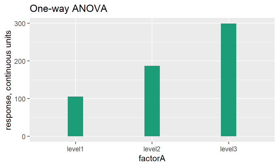
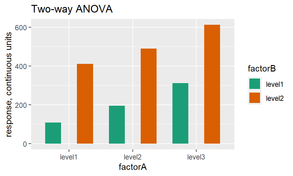
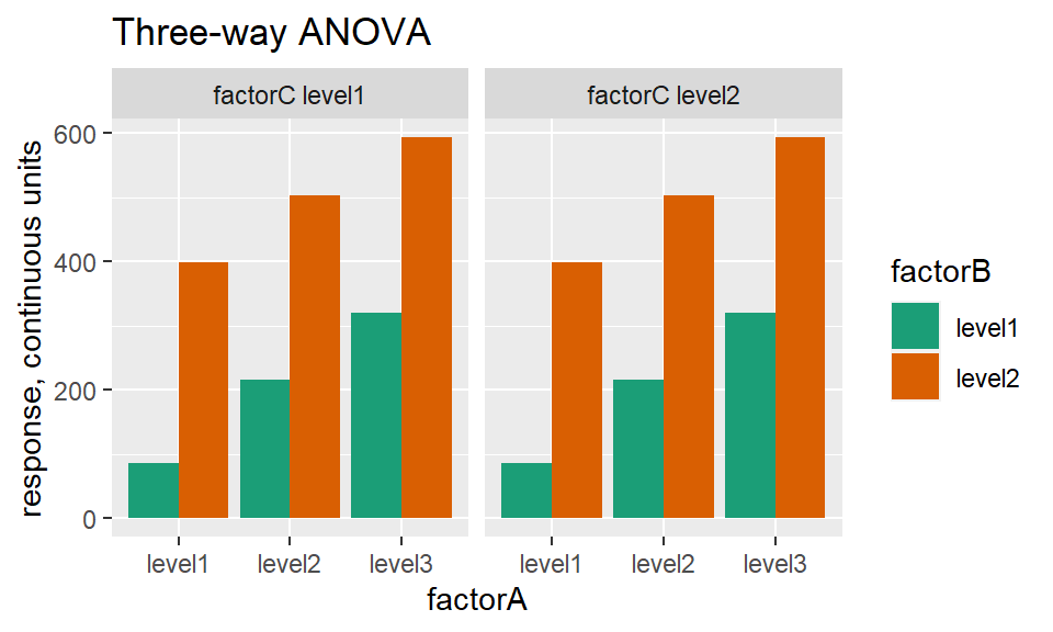
Figure 28.2: Typical graphs depicting some of the different ANOVA designs.

28.3 Why is ANOVA so common?

28.3.1 First, ANOVA is versatile.

One or more factors, each at several levels, can be tested simultaneously. We can test for the main effect of each factor, or for interactions between factors. We can also test for differences between specific individual groups within a context of many other groups, using post hoc analysis. Designs involving multiple intrinsically-related measurements from a common replicate are readily accommodated. We can have mixed designs where one factor is completely randomized and another is related measure within a single multi-factor experiments.

28.3.2 Second, ANOVA is efficient.

As a general rule, fewer replicates are needed to make the same number of pairwise group comparisons than would otherwise be necessary using a t-test-based experimental design. That efficiency can improve modestly as the number of groups increases.

28.3.3 Third, we can test many hypotheses simultaneously or a grand hypothesis.

Since each individual hypothesis test carries a risk of type1 error, ANOVA is a protocol to detect differences between many groups while ensuring that the overall type1 error, the so-called experiment-wise error or the family-wise error rate (FWER), won’t inflate to intolerable levels.

28.4 Jargon: Factors and levels

In jargon, ANOVA independent variables are classified as “factors.” ANOVA designs are said to be “factorial.” They are multifactorial if more than a single factor is involved, as in two-way and three-way ANOVA.

In other corners, ANOVA is referred to as factorial analysis (which should not be confused with factor analysis). Where some people describe an ANOVA experiment as a “one-way ANOVA” others might describe it as “one-factor ANOVA.” Elsewhere ANOVA is synonymous with multiple regression.

The factors of ANOVA represent categorical, discrete variables that are each applied at two or more levels. For example, a factor at three levels is an independent variable that has three discrete values.

Imagine an experiment to explore how a particular gene influences blood glucose levels. Blood glucose levels, a continuous variable, are measured in subjects that have three different genotypes for the gene: either wild-type, or heterozygous knockouts, or homozygous knockouts. Here, genotype is a discrete independent variable, a factor, which has three levels.

28.4.1 Working with factors in R

R requires that the ANOVA independent variables are classified as factors in data sets. The following text illustrates various ways to convert variables to factors.

The following script creates a vector object called genotype. By default, the data class for the genotype vector is character because it is comprised of character strings.

genotype <- c("wild-type", "heterozygote", "homozygote")
class(genotype)

## [1] "character"

To use genotype

We will need to convert the genotype object to a factor in order to use it.

If adding the genotype vector to a dataframe, just use a stringsAsFactors = T argument.

my.factors <- data.frame(genotype, stringsAsFactors = T)
str(my.factors)

## 'data.frame':    3 obs. of  1 variable:
##  $ genotype: Factor w/ 3 levels "heterozygote",..: 3 1 2

Sometimes levels of a factor in an experiment are represented by numeric values. To illustrate what I mean by this, imagine adding a second factor to the genotype experiment.

We wish to test for the effect of an antidiabetic drug on blood glucose at 0, 10 and 30 microgram/kg. These effects would be measured at each level of the genotype factor, leading to a nifty 3 X 3 factorial design.

We would create the vector drug as an object representing the drug variable and its three levels as follows. Note however that here, R does not coerce numeric values as factors:

drug <- c(0, 10, 30)
my.factors <- data.frame(genotype, drug)
str(my.factors)

## 'data.frame':    3 obs. of  2 variables:
##  $ genotype: chr  "wild-type" "heterozygote" "homozygote"
##  $ drug    : num  0 10 30

class(drug)

## [1] "numeric"

That’s easily fixed using the base as.factor function or forcats::as_factor function. Whatev.

drug <- as.factor(c(0, 10, 30))
genotype <- forcats::as_factor(genotype)
my.factors <- data.frame(genotype, drug)
str(my.factors)

## 'data.frame':    3 obs. of  2 variables:
##  $ genotype: Factor w/ 3 levels "wild-type","heterozygote",..: 1 2 3
##  $ drug    : Factor w/ 3 levels "0","10","30": 1 2 3

class(drug)

## [1] "factor"

Alternately, we would enter the drug levels as character strings (tossing in some other random character value):

drug <- as_factor(c("zero", "dark", "thirty"))
str(drug)

##  Factor w/ 3 levels "zero","dark",..: 1 2 3

We can do ANOVA with continuous independent variables. We just have to treat them as factors.

When a continuous independent variable is used at many levels (eg, a time series, a dose series, etc), regression per se can be a better alternative to ANOVA. Regression allows for capturing additional information encoded within continuous variables (eg, slops, intercepts, rate constants, half-lives, etc).

But that decision is more scientific than it is statistical.

If R’s anova functions are barking a confusing error message at us, we probably forget to factorize our variables.

28.5 ANOVA models: One-, Two-, and Three-way

If an experiment has only one factor, it is a one-way ANOVA design (alternately, “one-factor ANOVA”).

If an experiment has two factors, it is a two-way ANOVA or two factor design.

Three factors? Three-way ANOVA.

All of these models can also be either completely randomized, repeated/related measures, or mixed.

In a completely randomized structure, every level of the factor(s) is randomly assigned to replicates. Every replicate measurement is independent from all others. The two group analog is the unpaired t-test.

In a related measures structure, measurements within an experimental unit are intrinsically-linked. Every replicate receives all levels of a factor (eg, before-after, stepped dosing, or when subjects are highly homogeneous, such as cultured cells or inbred animals, or repeated recording from the same cell, etc).

The following give chapters each have a worked example for the five most common ANOVA experimental designs:

• One-way ANOVA completely randomized
• One-way ANOVA repeated measures
• Two-way ANOVA completely randomize
• Two-way ANOVA repeated measures
• Two-way ANOVA mixed CR/RM

Designs with more than two factors can be difficult to interpret using ANOVA.

Three-way ANOVA, for example, allows for such a large number of hypotheses to be tested simultaneously (three different main effects and four possible interaction effects, not to mention the large number of post hoc group comparisons) that it can be difficult to conclude exactly which factor at what level is responsible for any observed effects.

These larger designs also tend to break the efficiency rule, it’s fair to say that three way ANOVA designs tend to be over-ambitious experiments…over-designed and often under powered for the large number of hypotheses they can test. As a general rule, I advise against doing them.

Designing an experiment as completely randomized or related measures is largely a scientific, not a statistical, decision. Measurements are either intrinsically-linked or they are not based upon the nature of the biological material that we have at hand. Or because of the way the experiment is being conducted. When we’ve concluded that measurements are intrinsically-linked, then the choice must be a related measures design and analysis.

Similarly, choosing to run experiments as one-way or two-way ANOVA designs is also scientific.

In fact, we choose a two-way design mostly to test whether two factors interact. If not interested in the interaction, why combine two factors in one experiment? The main effect questions may be more safely answered using separate one-way ANOVAs, instead.

We’ll discuss interaction hypotheses and effects in more detail when we arrive at our two-way ANOVA discussion in the course.

28.6 Inference

ANOVA can be used inferentially as stand alone test for the main effect of a factor (or interaction effect between factors). More commonly, ANOVA is used as an omnibus test for permission to explore group differences using post hoc tests.

A positive ANOVA test result can be used to infer whether a factor, or an interaction between factors, is effective.

Continuing with the blood glucose example, we can use a positive F-test to conclude that genotype at a given locus influences blood glucose. And just leave it at that, without demonstrating which levels of the genotype differ from each other. I would write it up as follows: The genotype influences blood glucose (one-way related measures ANOVA, F(2,15)=11.48, p=0.0009). Then I will point to the data, which will speak for itself revealing which groups actually differ.

Alternately, a positive F-test result can be used as an omnibus. Here, a positive F-test implies that at least two levels of a factor differ from each other. The positive F-test grants us access to finding exactly where those differences exist. This is done by making posthoc pairwise comparisons.

We would, perhaps, compare each of the responses to the three genotypes to each other; for a total of 3 t-test like comparisons. I would adjust the p-values of each of those outcomes to control the FWER for those multiple comparisons.

The decision to use the F-test as a stand alone or as an omnibus is driven by our scientific objectives.

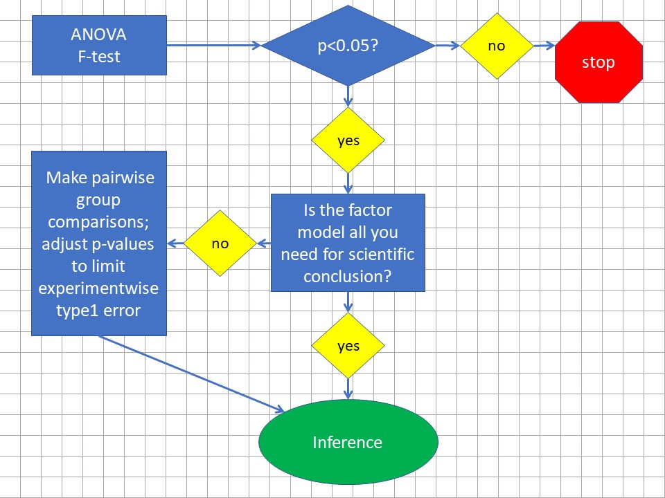
Figure 28.3: ANOVA work flow at a 5% type1 error threshold.

28.6.1 A quick peek at posthoc testing

These “post hoc” comparisons are, essentially, any of several variations on the t-test that are performed simultaneously. See Chapter 35 for more information about these.

Posthoc comparisons are designed in a way to limit the FWER to the predetermined type1 error threshold. Instead of all 5% error being devoted to compare two groups, the 5% is distributed across many comparisons. Sometimes dozens or more.

Unplanned is comparing all levels of all factors to each other. We might do that if we are looking for any and all differences on a project that is more exploratory in scope, such as in a hit screen.

Planned comparisons focus in on a much more limited subset of groups. We do this when the experiment is designed to test a fairly specific hypothesis or group of hypotheses.

What is important, statistically, is to make adjustments to the p-value threshold given all the comparisons made, so that the overall experiment-wise type1 error does not exceed our declared threshold (usually 5%).

In an experiment with \(k\) groups a total of \(m=\frac{k(k-1)}{2}\) possible group comparisons can be made.

Let’s use the simplest case of a \(k=3\) groups ANOVA as an example, such as the glucose genotype discussed above.

There are \(m=\frac{3(3-1)}{2}=3\) comparisons that can be made. Using the Bonferroni correction (\(\alpha_{adjust}=\frac{0.05}{m}=0.01667\)) the per comparison type1 error threshold is now 0.01667.

Thus, our adjusted threshold for declaring a statistical difference between 2 groups is now p < 0.01667, rather than p < 0.05.

If doing the 3 X 3 two-way ANOVA with genotype and drug as two factors, we now have \(k=9\) groups, yielding 36 possible comparisons and the threshold \(\alpha_{adjust}=\frac{0.05}{m}=0.001389\) for each comparison.

28.7 ANOVA calculations

The simplest way to think about ANOVA is that it operates like a variance budgeting tool. In the final analysis, the more variance associated with the grouping factor(s) compared to the residual variance, the more likely that some group means will differ.

ANOVA uses the least squares method to derive and account for sources of variation within a data set.

Recall, our measurements of the random variable \(Y\) having values of \(y_i\) for \(i=1, 2,..n\) and a sample mean \(\bar y\). Variance is calculated by dividing the sum of its squared deviates, \(SS\), by the sample degrees of freedom (df).

\[var(Y)=\frac{\sum_{i=1}^n(y_i-\bar y)^2}{n-1}=\frac{SS}{df}=MS\]

In ANOVA jargon the variance is also commonly referred to as the mean square \(MS\). This jargon emphasizes that variance can be thought of as an averaged deviation for measurements in a sample from their mean values.

That formula only illustrates how variance is calculated for a single sample group. What about multiple groups? As you might imagine, we have to incorporate information from all of the groups.

To begin to understand that, recognize that all ANOVAs, irrespective of the specific design are assumed to have two fundamental sources of variation:

1. Variation due to the experimental model, which is determined by the nature of responses to the independent variables.
2. Residual variation, which is variation that cannot be explained by the independent variables.

Law of Conservation of SS: That total variation within an experiment can be expressed as the sum of the squared deviates for these two sources. \[SS_{total}=SS_{model}+SS_{residual} \]

Let’s imagine a simple one-way completely randomized ANOVA data set that looks like the graph below. There is only one factor, which has three levels. Each of the 3 groups has five independent replicates, for a total of 15 replicates within the entire experiment.

Our model seeks to account for the effect of genotype \[SS_{model}=SS_{genotype} \]

Models are perfect but data are not. Not every data point is equal to the value of the black bar it is near. The residual variation are these differences and thus \[SS_{total}=SS_{genotype}+SS_{residual}\]

The graph illustrates each data point, the means for each group (black bars) and the grand mean of the sample (gold bars).

We can readily imagine the distances from the data points to the grand mean.

We can readily imagine the distances from the data points to the group means.

One can also appreciate and the distances from the group means to the grand mean.

We probably have a harder time visualizing the squares of those distances. My mind sees it Euclidean (geometrically). Larger distances, squared, lead to bigger boxes! The bigger the boxes, the greater that replicate contributes to the variance.

With that picture in mind, think of the variances within the experiment as follows:

• Total variance: average squared distances of the all the points to the grand mean
• Model variance: weighted average squared distances of group means to the grand mean
• Residual variance: average squared distances of the points to the group means

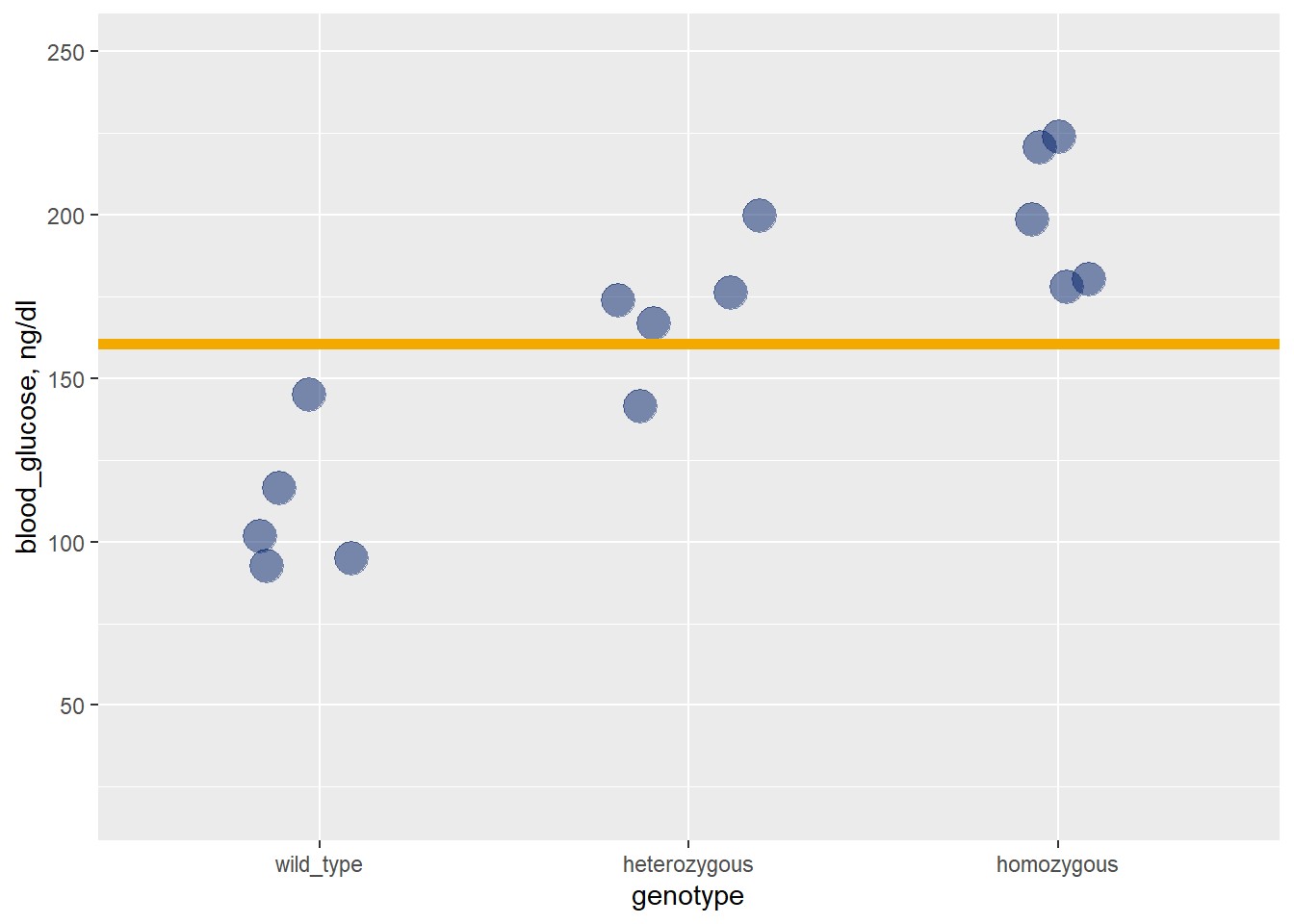
Figure 28.4: A completely randomized one way ANOVA, the genotype factor has three levels. Gold bar = grand mean, black bar = group means

28.7.1 Sums of Squares partitioning

The first step in an ANOVA involves partitioning the variation in a data set using sums of squares.

In this experiment, there are \(i=1, 2,...n\) independent replicates. There are also \(j=1, 2,...k\) groups.

The total sum of squares is the sum of the squared deviation from all data points to \(\hat y\), which represents the grand mean of the sample.

\[SS_{total}=\sum_{j=1}^k\sum_{i=1}^n(y_i-\hat y)^2\]

The sum of squares for the genotype effect is sum of the weighted squared deviation between the group means, \(\bar y_j\) and the grand mean. Here, \(n_j\) is the sample size within the \(j^{th}\) group. Thus, the group sample sizes are creating that weight.

\[SS_{genotype}=\sum_{j=1}^kn_j(\bar y_j-\hat y)^2\]

Anova software usually refers to this variation as the “treatment” sum of squares.

Finally, the residual sum of squares is calculated as the sum of the squared deviation between replicate values and group means,

\[SS_{residual}=\sum_{j=1}^k\sum_{i=1}^n(y_i-\bar y_j)^2\]

which, because the total variation amount of is fixed, can also be calculated as follows:

\[SS_{residual}=SS_{total}-SS_{genotype}\]

Software will tend to label this as either residual variation or as “error.” The term “error” arises from ANOVA theory, which holds that the true population means represented by these sample groups are “fixed” in the population. Thus, any deviation from the means is explained by random error.

Residual is jargon for the measurements of that “error.”

Perhaps we can intuit a few things.

First, the residual variation is the variation unaccounted for by the model. Meaning that whatever its causes, they are not under experimental control. If the data were perfectly explained by the model, every data point would be identical to a value of a group mean.

Second, if the variation around each group mean remains the same, but as the group means differ from each other more and more, the greater the fraction of the overall variation that will be associated with the model, and the less that will be associated with the residual.

Third, when the noise around those group means increases, less of the total variation will be associated with the model of group means, and the more with the residual.

In other words, big effect sizes are easier to detect, while noisy experiments tend to hide detectable differences between means, whereas clean experiments favor detecting these differences.

If this seems bloody obvious, and it is simple, then we should not have any problem processing how ANOVA works.

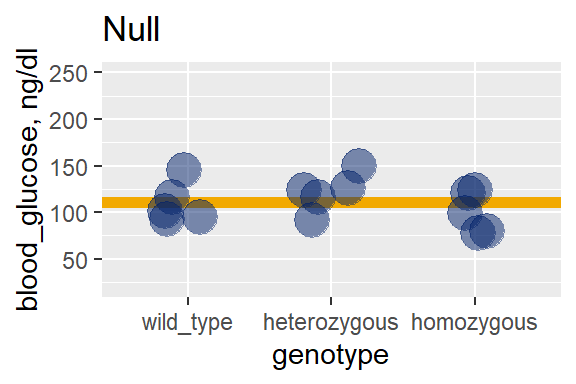
The following two graphs emphasize these observations. In the null graph, the group means are roughly equivalent and very nearly the same as the grand mean. There’s very little model variation relative to the grand mean. Most of the variation is in the residuals, relative to each group mean.

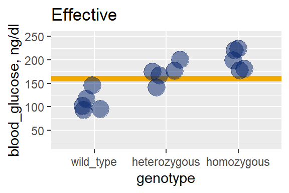
In the effective treatment graph, where the means truly differ because I coded them to differ, the residual variation is about the same as the null. The distance from each point to its group mean is about the same as in the null case.

But we can see there is a lot more model variation, at least compared to the null graph: The group means (black bars) really separate from the grand mean (gold line).

ANOVA tests become very simple when we understand this. The variation associated with the model is the signal and the residual variation is the noise. F tests are simple ratios between the model variance (or elements of the model) and residual variance. F tests are simple signal-to-noise ratios, just like every other statistical test.

28.7.2 The ANOVA table

The typical ANOVA table lists the following:

• source of variation,
• its \(df\),
• its \(SS\),
• its \(MS\)
• an F-test, where appropriate
• a p-value from the F-test

ANOVA functions in R vary in their output. But here’s the ANOVA table output for the data in the last previous figure:

anova(lm(blood_glucose ~ genotype, data))

## Analysis of Variance Table
## 
## Response: blood_glucose
##           Df  Sum Sq Mean Sq F value    Pr(>F)    
## genotype   2 21176.9 10588.4  22.979 7.877e-05 ***
## Residuals 12  5529.4   460.8                      
## ---
## Signif. codes:  0 '***' 0.001 '**' 0.01 '*' 0.05 '.' 0.1 ' ' 1

28.7.2.1 Sums of squares

As described above. These are the absolute measures of variation or deviation. Their values are in squared units of the response variable. Weird. But all \(SS\) sources will sum to \(SS_{total}\) and that is helpful.

28.7.2.2 Degrees of freedom

Variance is averaged deviation. The \(SS\) averaged. To calculate a variance we’ll need to divide the sum of squares by the degrees of freedom for that sum of squares. Just as sum of squares are calculated differently depending on whether it is total, or model or residual, so too are degrees of freedom.

The mathematical theory behind \(df\) is a bit more complicated than this, but as a general rule, we lose a degree of freedom every time the calculation of a mean is involved in determination of a given \(SS\). The basic idea is this: For that mean value to be true, one of the values used in the calculation must remain fixed, while all the others are free to vary.

The degrees of freedom for total variance are \(df_{total}=N-1\). We use all 15 replicates, \(N\), to calculate the grand mean \(\hat y\). One degree of freedom is lost for that grand mean to be true, one of those replicate values must be fixed while the others are free to vary.

We have \(k\) independent levels. The degrees of freedom for the genotype model variance are \(df_{genotype}=k-1\), because the \(SS_{model}\) calculation is based upon the group means, the value of one group mean must be fixed while two are free to vary.

The residual degrees of freedom are \(df_{residual}=N-k\) because although residual values are calculated for each data point, one degree of freedom is lost to calculate each group mean.

28.7.2.3 The mean squares

The mean squares are ANOVA jargon to represent variances. Think of variance as averaged variation or averaged deviation.

Total variance is \[MS_{total}=\frac{SS_{total}}{df_{total}} \]

The variance associated with the model is \[MS_{model}=\frac{SS_{model}}{df_{model}} \]

And the residual variance is \[MS_{residual}=\frac{SS_{residual}}{df_{residual}} \]

28.7.2.4 The F statistic and p-value

The null distributions of the F statistic are explained in Chapter 29.

The value of F is the ratio of two variances. For the result in the ANOVA table above \(F_{2,12}=\frac{10588.4}{460.8}=22.979\).

We can interpret that as saying the variance associated with the genotype model is 22.979-fold greater than the residual variance.

But is an F-statistic value of 22.979 with 2 and 12 degrees of freedom extreme?

The p-value is derived from an null F probability distribution that has 2 and 12 degrees of freedom. The p-value result in the table (Pr(>F)) is obtained using R’s pf function:

pf(22.979, 2, 12, lower.tail=F)

## [1] 7.87784e-05

The example above is a simple one factor completely randomized model for which there is only one F test, because it has only one component. Experimental designs that have more components, such as two or more factors with our without related measures, will have more F tests if completely randomized. A three-way ANOVA performed a certain way can have about a dozen F tests.

28.7.3 Post-hoc group comparisons

A positive ANOVA F test only tells you that the model (or its component) explains the response better than null.

The final stage of ANOVA, which is optional but done very commonly, is to run what are essentially t-test-like comparisons between groups. These posthoc tests help identify the specific factor levels that actually differ from each other.

The total number of comparisons that could be made are \(\frac{k(k-1)}{2}\). Sometimes we are fishing and want to do just that. Other times, for scientific reasons, only a specific subset are of any interest. For example, we would only want to compare test groups to a negative control group.

There are several ways to run these post-hoc group comparisons. See Chapter 35 for more information about these various options.

What is most important, however, is these be done in a way that keeps the family-wise error rate (FWER) below the pre-set type1 error threshold. That threshold is commonly 5% in biomedical research, but its value can be whatever you decide.

When would we change that threshold? Consider when we are conducting an exploratory “hit” screen involving large numbers of groups. For example, we have a lot of RNAseq data. Scientifically the mistake of throwing away false negatives might be worse than the mistake of accepting false positives. In that case, raising the type1 error threshold to 10% has merit.

28.8 Completely randomized or related measures

Related measures (RM) ANOVA is done when the measurements are not completely independent, but instead are intrinsically-linked.

Examples of intrinsically-linked subjects include

• two measurements, one from each of a pair of identical human twins,
• before and after on a single subject,
• all plates and wells from a single batch or passage of a cell culture,
• a protein preparation from a single batch,
• a single cell in culture,
• split tissues from one animal subject, and
• litter mates of isogenic animal strains.

There are certainly others.

An RM design involves taking multiple measurements from each independent replicate. Each replicate may vary randomly. That random variation between replicates can be accounted for, too. Because we can account for the variation within each replicate, that source of variation is no longer in the residual error term, but can be taken right into the model.

28.8.1 The problem of lost data in related measures designs

The CR vs RM design decision has a few important consequences.

First, when within-subject correlation is high, RM are much more efficient and less costly to produce. How much more? You can run Monte Carlo simulations to establish this for virtually any set of conditions you can imagine.

Second, over the course of any experiment it is possible to lose specific response values here and there. For example, a data value may be lost due to a bad lane in a replicate western blot, or we accidentally throw away a tube from a series, or we have a spill, or any of a number of such primitive errors.

CR ANOVA is tolerant of such losses. That leads to a missing replicate, and an unbalanced data sets, but it’s only one or a few values out of many.

That is not always the case with related measures designs. All of the values for every level of every factor for every replicate must be included for the analysis. If any values are missing for a given replicate, all of the remaining values for that replicate either have to be censored, or the missing values should be imputed.

The missing data problem becomes amplified in two way and three way related measures ANOVA. Those experiments tend to have more groups, meaning more data is at risk of being censored.

Researchers often ask if it is reasonable to ‘flip’ to a completely randomized analysis when they notice too many values are missing from their data set.

No, it is not reasonable. In fact, that’s a horrible p-value hack. The type of experimental design is scientifically-driven. Intrinsically-linked measurements are not independent, and should not be analyzed as if they are independent. To do so violates one of the two primary assumptions of the statistical analysis.

How to avoid this problem?

First, where possible, include an extra replicate or two as a hedge over what the power analysis suggests is necessary.

Second, don’t make a RM design too over-ambitious. Limit the number of levels to those that are scientifically important.

Third, be aware of the risk of lost values. Is the experimental protocol difficult? Are any protocol steps at high risk of failure? Are there any intrinsic barriers to efficiently collecting the data?

28.9 Two-way ANOVA

This is a method to investigate the effects of two factors simultaneously. Thus, the variation associated with each factor can be partitioned. This also allows for assessing the variation associated with an interaction between the two factors.

What is an interaction? Simply, it is a response that is greater (or lesser) than the sum of the two factors combined.

Let’s go back to the genotype blood_glucose problem. We’ll add a factor, and simplify the study a bit. We’re interested in a gene that, when absent, raises blood glucose. We’re also interested in a drug that, when present, lowers blood glucose.

We have reason to hypothesize that a genotype:drug interaction might exist. For example, the gene might encode a protein that metabolizes our drug, thus impairing the drug’s ability to lower blood glucose.

We’ll simulate a \(2\times 2\) experiment that has only the presence or absence of each of these factors.

Here’s the data:

set.seed(12345)
blood_glucose <- round(c(rnorm(5, 100, 20), rnorm(5, 75, 20), rnorm(5, 200, 20), rnorm(5, 100, 20)), 1)
drug <- as.factor(rep(rep(c(0, 30),each=5),2))
genotype <- rep(c("WT", "KO"), each=10)

test <- data.frame(genotype, drug, blood_glucose)

y0 <- mean(subset(test, genotype=="WT" & drug==0)$blood_glucose)
y30 <- mean(subset(test, genotype=="WT" & drug==30)$blood_glucose)
yend0 <- mean(subset(test, genotype=="KO" & drug==0)$blood_glucose)
yend30 <- mean(subset(test, genotype=="KO" & drug==30)$blood_glucose)
  
ggplot(test, aes(genotype, blood_glucose, color=drug))+
  geom_jitter(size=6, width =0.3)+
  scale_color_brewer(palette="Dark2")+
  stat_summary(fun=mean, geom="point", shape = 95, size= 15)+
  scale_x_discrete(limits=c("WT", "KO"))+
  labs(y="blood glucose")+
  geom_segment(aes(x="WT", y=y30, xend="KO", yend=yend30))+
  geom_segment(aes(x="WT", y=y0, xend="KO", yend=yend0))

## Warning: Computation failed in `stat_summary()`:
## Can't convert a double vector to function

## Warning in (function (kind = NULL, normal.kind = NULL, sample.kind = NULL) :
## non-uniform 'Rounding' sampler used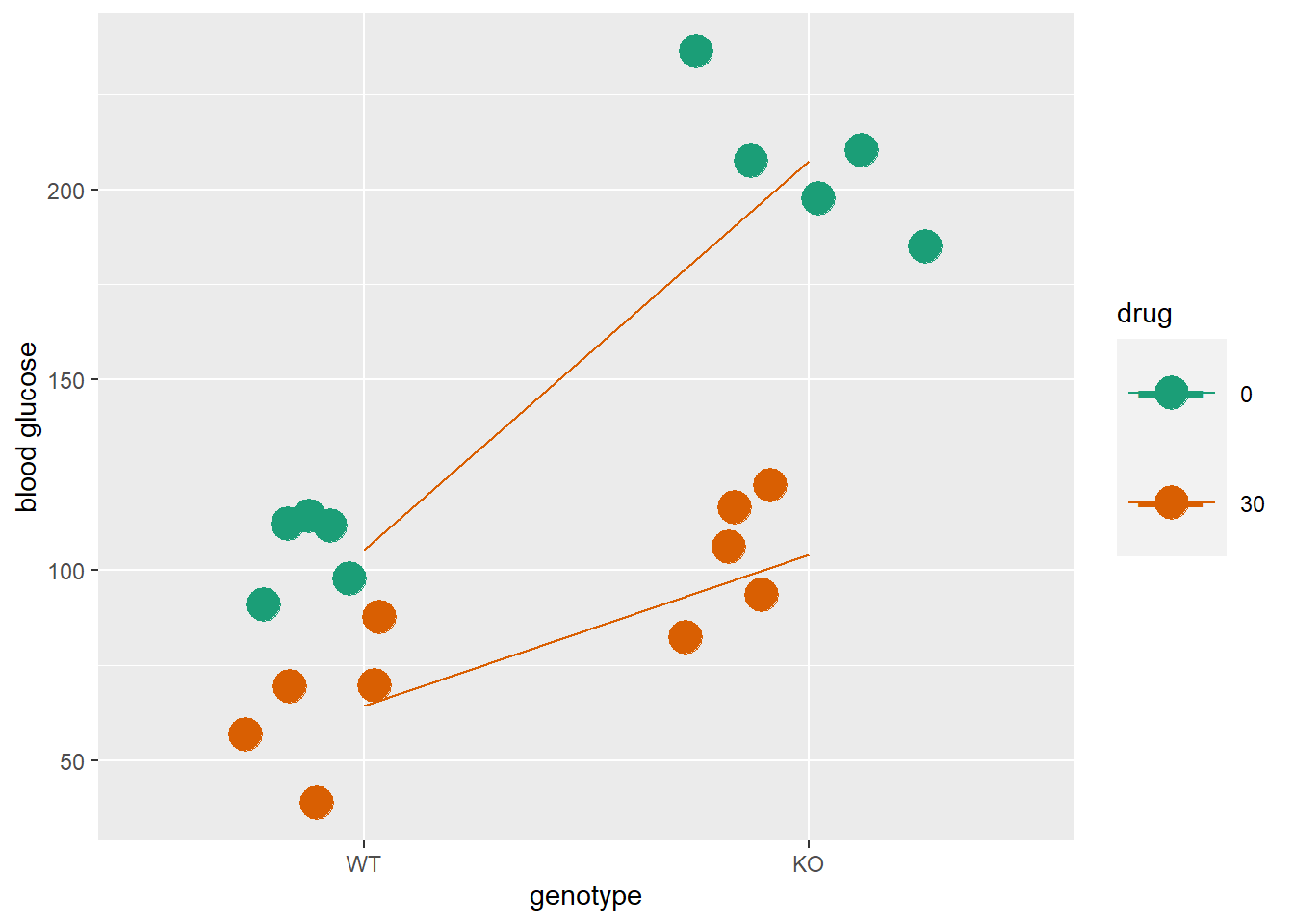

An interaction effect can be represented by the differing slopes of those two lines. If the lines are not parallel, it means that the effect of the drug is not the same at both levels of genotype. Or you could say the effect of the genotype is not the same at both levels of the drug. Whatever.

The statistical term used to describe such phenomena is that the two factors interacted.

Thus, a statistical interaction occurs when the effects of two factors are not the same across all of their levels.

Here’s a quick ANOVA table for those data. It has an F test for each of the factors genotype and drug, and an F test for the genotype:drug interaction. All three F-tests are extreme.

anova(lm(blood_glucose ~ genotype + drug +genotype*drug, test))

## Analysis of Variance Table
## 
## Response: blood_glucose
##               Df  Sum Sq Mean Sq F value    Pr(>F)    
## genotype       1 25127.0 25127.0  94.333 4.116e-08 ***
## drug           1 26028.1 26028.1  97.716 3.225e-08 ***
## genotype:drug  1  4845.4  4845.4  18.191 0.0005923 ***
## Residuals     16  4261.8   266.4                      
## ---
## Signif. codes:  0 '***' 0.001 '**' 0.01 '*' 0.05 '.' 0.1 ' ' 1

Since the F-test for the genotype:drug interaction is extreme, we can reject the null that there is no interaction between them. Furthermore, the existence of the interaction effect complicates the interpretation of the effects of the genotype and drug factors. Generally, an interaction effect supersedes an effect of either factor, alone.

Although genotype seems to have a strong effect on glucose levels, that’s really blunted in the presence of drug. And although the drug seems to reduce glucose, that effect becomes remarkably prominent when the genotype changes. When interactions occur, the effect of one factor cannot be interpreted without condition on the other factor!

It might be useful to see the data for the discussion that follows.

genotype	drug	blood_glucose
WT	0	111.7
WT	0	114.2
WT	0	97.8
WT	0	90.9
WT	0	112.1
WT	30	38.6
WT	30	87.6
WT	30	69.5
WT	30	69.3
WT	30	56.6
KO	0	197.7
KO	0	236.3
KO	0	207.4
KO	0	210.4
KO	0	185.0
KO	30	116.3
KO	30	82.3
KO	30	93.4
KO	30	122.4
KO	30	106.0

Four sources of variation are accounted for: the main effect of genotype, the main effect of drug, the interaction between drug and genotype, and the residual error.

Three F tests were performed. Each of these used \(MS_{residual}\) in the denominator and the \(MS\) for the respective source in the numerator.

How has this variation been determined?

The experimental model is as follows: \[SS_{model}=SS_{genotype}+SS_{drug}+SS_{genotype\times drug} \]

The grand mean of all the data is computed as before: \[\hat y=\frac{1}{n}\sum_{i=1}^ny_i \]

There are two factors, each at two levels. Thus, there are a total of \(j=4\) experimental groups. Each group has a sample size of \(n_j=5\) replicates and represent a combination of independent variables: WT/0, WT/30, KO/0, KO/30. The mean of each group is \(\bar y_j\).

Therefore, \[SS_{model}= \sum_{j=1}^kn_j(\bar y_j-\hat y)^2 \] represents the total model variation.

We can also artificially group these factors and levels further. Two groups correspond to the levels of the genotype factors and two correspond to the levels of the drug factor. Their means are \(\bar y_{wt}, \bar y_{ko}\) and \(\bar y_0, \bar y_{30}\), respectively. Each of these groups has a sample size of \(2n_j\).

These contrived means are used to isolate for the variation of each of the two factors:

\[SS_{genotype}= \sum n_{wt}(\bar y_{wt}-\hat y)^2+n_{ko}(\bar y_{ko}-\hat y)^2 \]

\[SS_{drug}= \sum n_{0}(\bar y_{0}-\hat y)^2+n_{30}(\bar y_{30}-\hat y)^2 \]

All that remains is to account for the variation associated with the interaction effect. That can be solved algebraically: \[SS_{genotype\times drug}=SS_{model}-SS_{genotype}-SS_{drug} \]

Because two way ANOVA’s have two factors, one of the factors can be applied completely randomized, and the other can be applied as related measures. Or both factors can be completely randomized, or both can be related measures.

28.10 Other ANOVA models

For all ANOVA experiments, irrespective of the design, the total amount of deviation in the data can be partitioned into model and residual terms:

\[SS_{total}=SS_{model}+ SS_{residual}\]

What’s interesting is that different ANOVA experimental designs have different models. We’re interested in two factors, factorA and factorB, and have the ability to study each at multiple levels. The interaction between factorA and factorB is \(A\times B\)

One way CR: \(SS_{model}=SS_{factorA}\)

One way RM: \(SS_{model}=SS_{factorA}+SS_{subj}\)

Two way CR: \(SS_{model}=SS_{factorA}+SS_{factorB}+SS_{A\times B}\)

Two way RM on A factor: \(SS_{model}=SS_A+SS_B+SS_{A\times B}+SS_{subj\times A}\)

Two way RM on both factors: \(SS_{model}=SS_A+SS_B+SS_{A\times B}+SS_{subj\times A}+SS_{subj\times B}+SS_{subj\times A\times B}\)

The big difference between completely randomized and related measure designs is that in the latter, we’re now accounting for the deviation associated with each replicate in the model! Otherwise, that replicate deviation would have been blended into the residuals.

This turns out to be a pretty big deal. When that deviation due to the subjects is pulled out of the residual, it lowers the value of the denominator of the F statistic. Thus making the F statistic larger!

28.10.1 R and ANOVA

There are a handful of ways to conduct ANOVA analysis on R. These are not necessarily more right or wrong than the others. What is important to know, however, is that they do perform calculations differently under certain circumstances (eg, Type 1 v Type 2 v Type 3 SS calculations). Therefore, they produce distinct results.

This always confuses researchers, particularly when comparing R’s results to other software we might be more comfortable with. We wonder which output is “right.” Chances are they are all “right.” We have that output because of the way we argued the analysis.

This again emphasizes the need to share specific details of the analysis in our publications. In this case, specify using R, specify the package version and the R function used, and even specify the arguments. Or append an R script file as supplemental information to illustrate exactly how the analysis is performed.

Given data and a group of arguments we’ll call foo, R’s ANOVA function options are as follows:

anova - A function in R’s base. eg, anova(lm(foo))

aov - A function in R’s base. eg, `aov(foo)

Anova - A function in R’s car package. eg, Anova(lm(foo))

ezAnova - A function in R’s ez package, ezAnova(foo)

There are others. For example, since ANOVA analyses are also general linear models the same basic problem can also be solved using lm(foo)without ANOVA. Passing an lm(foo) into an ANOVA function mostly just provides output in the familiar ANOVA notation. The statistical fundamentals of lm(foo) and ezAnova(foo)are identical.

For the ANOVA part of this course, we’ll use ezANOVA from the ez package. In particular, it is a bit more straightforward to use (and teach) in terms of arguing the experiment’s ANOVA model.

Key Jargon to understand to do ezANOVA in R

Specify a completely random design by defining the ‘between’ variable as your factor name. The between here is meant to imply comparisons between groups.

Specify a related measures design by defining the within variable as your factor name. The within here is meant to imply comparisons within replicates.

28.10.1.1 Type of calculation

When analyzing 2-way and 3-way ANOVA’s there are three different methods to calculate, which are referred to as type I, type II and type III.

When an experiment is balanced, which is to say it has equal sample sizes per group, the type of calculation is immaterial. In that case,type I, II and III yield exactly the same output.

Unbalanced experiments are those in which the sample sizes of groups are not the same. As long as the differences are not too large, the presence of unbalance is usually not a problem. But it will always impact the precise output of different ANOVA functions, depending upon whether they perform type I, II or III calculations.

This is what really causes confusion when we notice different output from different functions. This is particularly confusing when comparing the output of different ANOVA functions in R (eg, Anova vs aov vs anova vs ezAnova) and/or commercial software (eg, SAS, SPSS, Prism). The researcher scratches her head, wonders which is “correct.”

In one sense, they are all correct.

Type I, II and II sum of squares calculations are explained here.

Suffice to say this is important to not overlook. This serves to illustrate how providing good detail about the software used to analyze data is important for reproducibility.

The most significant point to understand is that some commercial software uses type 3 calculations by default. As a consequence, given the same data set, the results from those packages may not coincide perfectly with those of ezANOVA unless using a type = 3 argument in the function.

My recommendation is to use type = 2 when interested in only testing hypotheses about the main effects of factors, and there is no interest in an interaction if working on a two- or three-way ANOVA data set. That’s because type = 2 is purported to yield consistently higher power for main effects.

Use type = 3 when, instead, the experiment is designed to test whether an interaction occurs between factors. When an interaction occurs, the main effects are not interpretable.

Type I sum of squares are calculated when using the anova and aov functions of base R. This is otherwise known as “sequential” sum of squares calculation. On multifactor data with those functions, the results can differ given the order by which the factors are argued. Thus, aov(lm(outcome~factorA + factorB)) might yield slightly different results compared to aov(lm(outcome~factorB + factorA)). The idea is to calculate the effect on a factor that is most interesting to you scientifically, while “controlling” for the effect of the other factor.

When using ezANOVA we can explicitly argue which calculation we wish to run, removing some ambiguity about what actually happened.

28.11 Alternatives to ANOVA

When the outcome variable is measured and the design is completely randomized, the data can be analyzed using the general linear model using R’s lm function, rather than by ANOVA. This allows for analyzing interaction effects between factors. The results will be the same as ANOVA. If the design has a related measures component, then a linear mixed effects model should be run instead. In that case, use lmer in the lme4 package.

Alternately a nonparametric analysis can be performed using either the Kruskal-Wallis (completely randomized) for the Friedman (related measures) test. Bear in mind that no nonparametric analog for the two-way ANOVA exists. Thus, hypotheses related to interaction effects are not testable using nonparametric statistics.

Finally there is the generalized linear model (glm) for completely randomized designs or the generalized linear mixed model (glmer) for designs that incorporate related measures, respectively. Each of these allow for testing interactions between factors. The generalized linear models also allow for a flexible array of outcome variables. These should be used, rather than ANOVA, when the outcome variable is non-normal or is discrete. For example, these are the tools of choice when the outcome variable is binomial (logistic regression) or frequency data (Poisson regression) and there are 3 or more groups to compare. Additional families are possible.

28.11.1 Screw ANOVA, Just Tell Me How to t-Test Everything

OK, fine.

This is far from ideal because an ANOVA-free approach risks introducing bias through cherry-picking comparisons after unpacking the data (the HARK fallacy).

You don’t have to do ANOVA for an experiment with 3 or more groups (or anything else for that matter–you just have to be able to defend your choices). A major purpose of ANOVA is to maintain an experiment-wise type1 error of 5%. But there are other ways to accomplish this objective.

For example, you might skip the ANOVA step and simply run serial t-tests comparing all of the groups in an experiment. Or run t-tests to compare a pre-planned sublist of all possible comparisons. The emphasis here on pre-planning is important. Make decisions ahead of time about what is to be compared, then make only those comparisons. No more and no less. Otherwise, you’re snooping. Once you’re in snooping mode, you’re deeply biased towards opportunistic outcomes.

For example, you may run multiple control groups within your experiment to signal that some important aspect of the protocol is working properly, but these controls are otherwise not scientifically interesting (with respect to testing new hypotheses). You may not wish to expend any of your type1 error budget doing comparisons on these controls.

With those reservations noted, what follows are two ways to go about this.

To begin, if we have \(k\) levels of independent variables in our experiment it has a total of \(m=k(k-1)/2\) possible comparisons that could be made.

The pairwise.t.test is the function to use for this purpose. Use it to make the group comparisons that interest you. choosing the p.adjust.method that strikes your fancy. Two of the latter are listed below.

28.12 Summary

• We conduct ANOVA designed experiments intuitively, any time we have 3 or more groups.
• In R make sure that variable you want to be a factor is coded as a factor.
• Accounting for combinations of factors and whether the factor is applied randomized or related measures, We have at least 12 different ANOVA designs at our disposal.
• F-tests compare model variance to residual variance; if F is large, the model is extreme.
• ANOVA test results can infer effects of factors, or be permission for posthoc testing
• Several ANOVA methods exist in R. When configured the same, they should give the same output.