Chapter 39 Correlation
Something for your pipe: Having high confidence in a non-zero correlation is not the same as concluding a strong correlation exists!
library(tidyverse)Use correlation analysis to assess if two measured variables co-vary. If two variables co-vary they are said to be associated.
You’ll recall discussing the concept of association back when we dealt with discrete data. For example, an association between smoking and cancer could be tested by counting the frequency of cancers within a group of smokers, such as in a case-control design.
The main way correlation differs from these previous tests of association is that correlation analysis is conducted using measured rather than discrete (ie, counted) variables. For example, in a cancer study we might attempt to correlate lifetime levels of carcinogen exposure with age of cancer diagnosis. Here, both carcinogen levels and age are measured variables, and correlation analysis would be more appropriate than association analysis.
Correlation coefficients are effect sizes that are used as estimators of the correlation parameter, \(\rho\), of the sampled population.
Correlation coefficients estimate the strength and the direction of the linear relationship by which two variables co-vary.
Covariance estimates the strength of an association between two variables.
If two variables have a correlation coefficient of zero they do not co-vary; they are not associated; they are independent. An analog of the one sample t-test can be used to test the null hypothesis that a correlation coefficient is equal to zero.
39.1 Correlation != Causation
It is important to recognize that correlation gives no information about causality.
The reason is very simple. In a correlation analysis, when neither of the two variables is a true experimentally manipulated predictor variable causality cannot be determined. The two variables in a correlation analysis are each outcome variables (aka dependent variables).
Thus, it’s not possible to know from correlation analysis if brain size causes larger body size, or if larger body size causes larger brain size!
Please also pay particular attention to what a t-test on a correlation coefficient tells you. It’s not a test of an experimental hypothesis. It is not an inferential or causal hypothesis test. It simply tests whether a non-zero correlation exists between two variables.
Correlation is also not regression. Thus, the most proper way to illustrate correlation is to simply show the scatter plots of the data, without superimposing best-fit regression lines. Those lines imply a regression analysis was performed. Regression (and regression lines) should be reserved for when one of the variables is a true predictor variable and the intent is to model the values of the response variable at each level of predictor.
39.2 Correlation in Multivariate Outcomes and Paired Designs
Correlation is very important in many practical ways in biomedical research wherein predictor variables are deployed. It’s perhaps most important in multivariate experiments. These experiments generate two or more outcome variables from a single sample. These variables tend to be correlated.
For example, imagine a study that measures the expression of several different proteins, or several different mRNA’s, simultaneously at each level of some stimulus. All of these mRNA’s and proteins have an inherent correlation since they arise from identical stimulus conditions within given replicates. Their covariances are accounted for when using multivariate statistical methods (eg, MANOVA)
Correlation also creeps into experiments in more subtle but really important ways. For example, given their highly homogeneous nature, seemingly disparate variables measured in cell culture experiments and from laboratory mice often have striking underlying correlation. This correlation can and should be accounted for when planning experiments and analyzing their data.
We’ve seen a hints of this already in our discussions on paired t-tests and related measures ANOVA analysis. One reason those experimental designs are so efficient is because their analysis takes advantage of the underlying correlation structures within the subjects!
39.3 Correlation coefficients
The statistical parameters used to describe the correlation between two variables is the correlation coefficient. The three different correlation coefficients we’ll discuss are Pearson’s r, Spearman’s r_s and Kendall’s tau. Each arrives at roughly the same answer, but in different ways.
If you say to me, “The correlation between brain and body sizes is 0.489,” then I will ask, “Is that Pearson’s or Kendall’s or Spearman’s?”
39.3.1 Pearson’s correlation coefficient
The key assumptions are:
- The sample is random.
- Each replicate is independent of all other replicates.
- The measurements are derived from a population that has a bivariate normal distribution.
A bivariate normal distribution arises when two variables are each normally distributed. With small sample sizes we can’t really know if this latter assumption is met. However, we can safely assume this assumption if both variables have been measured in their linear range.
The Pearson correlation coefficient estimates the strength of a linear association between two measured variables. It can be calculated from the paired variables X and Y which take on the values x_i and y_i for i=1 to n pairs:
\[r=\frac{\sum\limits_{i=1}^n(x_i-\bar x)(y_i-\bar y)}{\sqrt{{\sum\limits_{i=1}^n}(x_i-\bar x)^2}\sqrt{\sum\limits_{i=1}^n(y_i-\bar y)^2}}\]
The standard error of \(r\) is:
\[SE_r=\sqrt{\frac{1-r^2}{n-2}}\]
Covariance is the strength of association between two measured variables and is calculated as follows:
\[Covariance(X,Y)=\frac{\sum\limits_{i=1}^n(x_i-\bar x)(y_i-\bar y)}{n-1}\]
The magnitude of covariance is difficult to interpret because it depends upon the values of the variables. In contrast, the correlation coefficient can be thought of as a normalized covariance, and its magnitude therefore useful as an index of effect size.
The t-test for a correlation coefficient is:
\[t=\frac{r}{SE_r}\]
Two-sided null hypothesis: \(\rho=0\) One-sided null hypothesis: \(\rho\le0\) or \(\rho\ge0\)
39.3.1.0.1 Alternative formulas for Pearson’s correlation coefficient
\[r=\frac{Covariance(X,Y)}{s_x s_y}\], where \(s_x\) and \(s_y\) are the sample standard deviations for the variables \(X\) and \(Y\), respectively.
\[cor(X,Y)=\frac{cov(X,Y)}{\sqrt{var(X)var(Y)}}\]
39.3.2 Spearman’s rank correlation
- The sample is random
- Each replicate is independent of all other replicates
The word ‘rank’ should alert you that this is a non-parametric method.
Spearman’s approach to calculating correlation is used when bivariate normality cannot or should not be assumed, or for when one (or both) of the outcome variables is/are ordered data.
To calculate Spearman’s correlation coefficient, \(r_s\), first each of the variables are converted to ranks in the usual way. For example, a measured variable vector comprised of the values \(2, 4, 5, 5, 12,...\) is converted to the rank values \(1, 2, 3.5, 3.5, 5,...\). Note how ties are handled by conversion to mid-ranks.
As you can see below, Spearman’s correlation coefficient \(r_s\) is calculated in the same way as for Pearson’s, except that rank values are used instead.
Let the values \(v\) and \(w\) represent the rank values of the variables \(X\) and \(Y\), respectively:
\[r_s=\frac{\sum\limits_{i=1}^n(v_i-\bar v)(w_i-\bar w)}{\sqrt{{\sum\limits_{i=1}^n}(v_i-\bar v)^2}\sqrt{\sum\limits_{i=1}^n(w_i-\bar w)^2}}\]
Given a large sample size, a t-test can be used to test the null hypothesis that \(r_s\) differs from zero.
\[t=\frac{r_s}{SE_{r_s}}\], where \(SE_{r_s}=\sqrt{\frac{1-r^2_s}{n-2}}\)
Sources differ on what comprises a large sample size. In R, by default the cor.test function for the Spearman method uses a t-test when n>1289. Otherwise, the function generates an S statistic via permutation analysis, from which p-values are calculated. See ?cor.test for more details.
39.3.3 Kendall’s tau
Kendall’s is an alternative to Spearman’s and would be used if the bivariate normal assumption cannot be met.
In this procedure, the pairs are ordered on the basis of the rank values of the \(X\) variable. If \(X\) and \(Y\) were perfectly correlated, the rank values of the \(Y\) variable would be perfectly concordant with the ranks of the \(X\) variable. The number of concordant pairs, \(n_c\) and discordant pairs, \(n_d\) are then counted to derive the correlation coefficient, tau.
\[tau=\frac{n_c-n_d}{\frac{1}{2}n(n-1)}\]
As for Spearman’s, a posthoc test of null hypothesis that tau differs from zero can be calculated. P-values are calculated using exact tests for small sample sizes, or by standard normal approximation for larger sizes.
39.3.4 Which correlation method to use?
Obviously, given a single data set, one is now equipped to derive 3 separate correlation coefficient values using either Pearson, Spearman or Kendall methods. Which of the 3 estimates is “right?”
Use Pearson’s if the bivariate normal assumption can be met. Otherwise, choose Spearman’s or Kendall’s approach.
39.3.5 R correlation analysis functions
It is very easy to do correlation analysis in R, which requires two simple functions: cor and cor.test.
The former is used to only generate correlation coefficients, whereas the latter will generate these coefficients and also run posthoc “significance” tests.
Below, the random variables x and y are generated to illustrate uncorrelated data. Correlated data are illustrated by calculating the random variable z, from x and y, so that z has a pre-specified (in the example r = 0.9) correlation with y.
set.seed(12345)
r <- 0.9 #correlation coefficient between y and z
x <-  rnorm(300, 30, 2)
y <-  rnorm(300, 30, 2)
z <- r*y+sqrt(1-r^2)*x

spur <- data.frame(x, y, z)
39.3.6 Plot the correlations
One can readily see the “shotgun” pattern of an uncorrelated sample (blue) as opposed to the elliptical “galaxy” pattern in the correlated sample with greater centroid density.
spur %>% ggplot(aes(x, y)) +
  geom_point(color="#002878") +
  theme_bw() +
  geom_point(aes(z,y), color="#d28e00")+
  labs(x="x or z")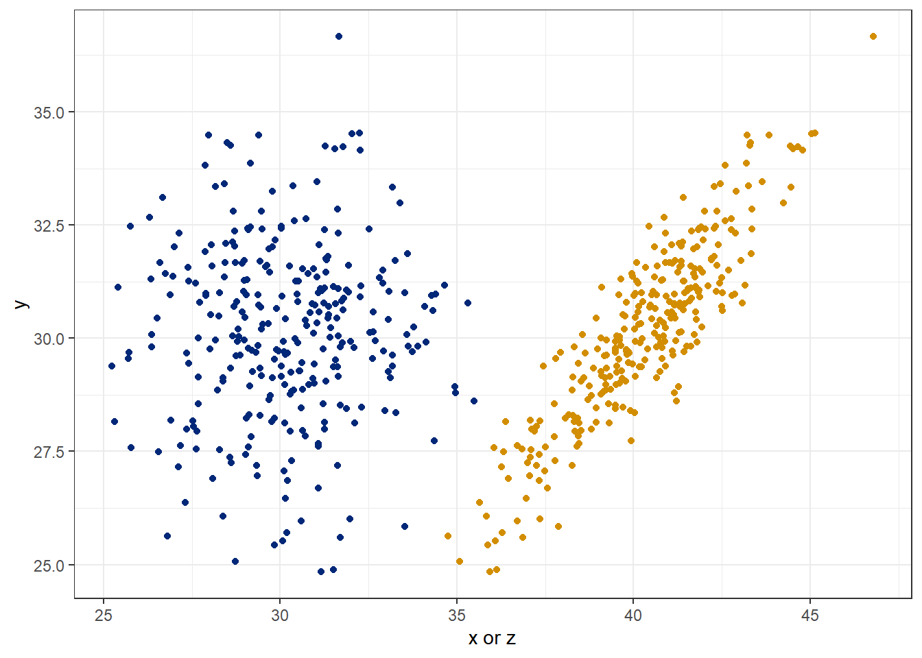
39.3.7 Calculate a correlation coefficient and posthoc test
The script below tidy’s up the simulated data from above. It then runs some calculations to compare outputs. Note how the output of the cor function can be replicated exactly by.hand. The functions cor, cov and var are each components of the basic stats package and have utilities in their own rights.
Notice how \(r\) and \(r_s\) give similar but different values. Not unexpected, they are different calculations!
The cor.test function will provide a confidence interval only for the pearson method.
X <- spur$x
Y <- spur$y
Z <- spur$z

cor(X, Y, method="pearson")
## [1] 0.02426448by.hand <- cov(X,Y)/sqrt(var(X)*var(Y)); by.hand## [1] 0.02426448cor(Z,Y, method="pearson")## [1] 0.8956038cor(Z, Y, method="spearman")## [1] 0.8648838cor.test(X, Y, method="pearson", alternative="two.sided", conf.level=0.95)##
## Pearson's product-moment correlation
##
## data: X and Y
## t = 0.41899, df = 298, p-value = 0.6755
## alternative hypothesis: true correlation is not equal to 0
## 95 percent confidence interval:
## -0.08922152 0.13712853
## sample estimates:
## cor
## 0.02426448cor.test(Z, Y, method="pearson", alternative="two.sided", conf.level=0.95)##
## Pearson's product-moment correlation
##
## data: Z and Y
## t = 34.754, df = 298, p-value < 2.2e-16
## alternative hypothesis: true correlation is not equal to 0
## 95 percent confidence interval:
## 0.8706648 0.9159499
## sample estimates:
## cor
## 0.895603839.3.8 Interpretation of correlation output
Two variables can either be positively correlated, or negatively correlated, or not correlated at all. Values for a correlation coefficient can range from -1 to +1, with the strongest correlations at either extreme, and weakest correlations at around zero. Thus, the correlation coefficient is a measure of effect size.
If the correlation coefficient differs from zero, the two variables are correlated, or are said to be associated. However, whether a particular value for a correlation coefficient should be considered strong or weak is usually a matter of scientific judgment.
The p-value should not be used as an expression of effect size. It is possible to have a very low p-value for weak correlation. In particular, large sample sizes can generate low p-values for rejecting the null of no correlation.
Remember, having high confidence in a non-zero correlation is not the same as concluding a strong correlation exists!
39.3.8.1 Write Up
The variables X and Y are uncorrelated (Pearson’s r=0.024, 95%CI= -0.089 to 0.137, p=0.6755).
The variables Z and Y are correlated (Pearson’s r=0.895, 95%CI=0.87 to 0.916, p<2.2e-16).