Chapter 46 Mixed model logistic regression
library(tidyverse)
library(lme4)
library(viridis)
library(multcomp)
library(broom)
A mixed model logistic regression is an appropriate test for experimental designs where paired/repeated/related measures are taken and the outcome variable is a proportion. In general, mixed model regression should be used when there is a heirarchical structure in the design yielding measurements that are non-independent.
Take for example an cell culture-based experiment. Independent replicates are performed. On a given day, working from a common batch of cells plated at the same time, none of the measurements from within a batch are independent of each other. However, we can assume that measurements collected between batches are independent.
The “mixed” in the title is jargon referring to the fact that the model has both fixed and random components. Which is more jargon to deconvolute, I suppose.
46.1 Mixed models, fixed and random effects
Brief synopsis, in regression jargon the fixed effects of an experiment are those represented by the intercept and by the predictor
Recall that statistical models are perfect, while data are not.
The fixed effects in a simple linear regression model are the ‘background’ level of the response in the system, estimated by the intercept coefficient \(\beta_0\), and those effects due to the predictor variable, which is estimated by the slope coefficient, \(\beta_1\). Here’s a simple linear model: \[Y=\beta_0+\beta_1X+\epsilon\]
Performing a regression on a data set allows us to generate estimates for these fixed effects based upon the behavior of a sample. The error term, \(\epsilon\) accounts for the residual differences between the points predicted by the model and the values for the actual data.
For example, let’s imagine we’re measuring whether a protein is in the nucleus or in the cytosol, as a binary dependent variable \(Y\). The experiment involes stimulating cultured cells with different types of mitogens \(X\). This condition is followed counting some number of cells and deciding how many show nuclear protein and how many cells show the protein in the cytosol. Furthermore, the experiment is replicated independently several times.
The word ‘fixed’ effects comes from assuming that the slopes and intercepts of the regression model have a fixed value in the wider populaton of cells that are sampled. A regression routine run on experimental data generates estimates for those fixed values.
We use these model coefficients to draw perfect lines or curves through some messy data. In the statistical model world the data are imperfect! That explains why we add a residual term to the model, so we can capture in it the stochastic deviation from the these fixed regression coefficients that the actual data has.
We learned way back in ANOVA about experimental designs where multiple measurements are derived from a given experimental unit. In such designs it becomes possible to attribute some of the residual error as the “random” variation among independent replicates. The jargon ‘random’ in regression is the same as the ‘repeated/related measures’ jargon used in ANOVA.
In other words, in a cell culture experiment, we would expect random variation between cell culture passages might affect nuclear location of the protein. This random variation could arise from anything, including the state of the cells and the preparation of fresh reagents.
But within a replicate we would expect those random variations to affect each cell culture well similarly.
We account for this repeated measure in our regression models as the “random” effect. The term comes from thinking that the replicate to replicate variation in a population is what is random. Usually, controlling for random effects in a model has the effect of lowering the stochastic residuals. By definition, these are the stochastic variation in the data unaccounted for by the random and fixed effects of a model.
Thus, mixed models have both fixed and random effects.
Here’s an example for a common experimental design for a logistic linear mixed model. The outcome response involves the researcher making a decision about whether the outcome variable belongs in one one category or another. And the responses to all of the treatment levels are measured within each independent replicate.
46.1.1 NFAT localization within smooth muscle cells
The NFAT transcription factors mediate gene expression responses under the control of mitogen signaling. In perfectly quiescent cells they are cytosolic. When cells are activated by stimuli that increase cytosolic calcium, the phosphatase calcineurin strips NFATs of phosphate groups, exposing a nuclear localization signal. The NFATs then translocate to the nucleus where they contribute to gene expression responses after binding to enhancer elements in genes.
Here’s a simple question: Can NFAT distinguish between different types of triggers that regulate calcium signaling? If so, this might be evident by measuring different degrees of nuclear translocation.
To assess NFAT activation directly, the ability of 3 different mitogens (AngII, UTP and PDGF) to cause nuclear translocation was measured and compared to a vehicle control. Cells in culture were treated with an agent for 30 min before they were fixed and stained with an NFAT antibody.
A blinded observer randomly selected a region and counted a total of one hundred cells on each plate. To determine the proportion showing nuclear NFAT the cells were scored as having mostly nuclear NFAT or mostly cytosolic NFAT. The experiment and counting procedure was replicated independently 5 times.
A few features of this design are notable: * The predictor variable is treatment at 4 levels (Veh, AngII, UTP and PDGF) * The outcome variable is discrete and has a binomial distribution (nuclear or cytoplasmic NFAT) * This is cell culture based. A replicate is defined as a day in which all stimuli were administered side-by-side on different wells from a common cell culture source passage. Therefore, within a replicate all counts are intrinsically-linked. The regression model will have a random term to account for this.
46.2 Data
The data are in a csv file. The treatment code is as follows: a=vehicle, b=AngII, c=UTP and d=PDGF.
data <- read.csv(file="datasets/smnfat.csv")Here’s a poor man’s heat plot of the data. The replicates are color-coded, so you can see that all of the cells counted from all of the replicates are represented.
ggplot(data, aes(x=treatment, y=as.factor(counts), color=reps))+
  geom_jitter(width=0.3, size=3, alpha=0.8)+
  scale_color_viridis(discrete=T) +
  scale_y_discrete("counts", labels=c("0"="Cyto", "1"="Nuc"))+
  scale_x_discrete("treatment", labels=c("a"="Veh", "b"="AngII", "c"="UTP", "d"="PDGF"))+
  theme_classic()
## Warning in (function (kind = NULL, normal.kind = NULL, sample.kind = NULL) :
## non-uniform 'Rounding' sampler used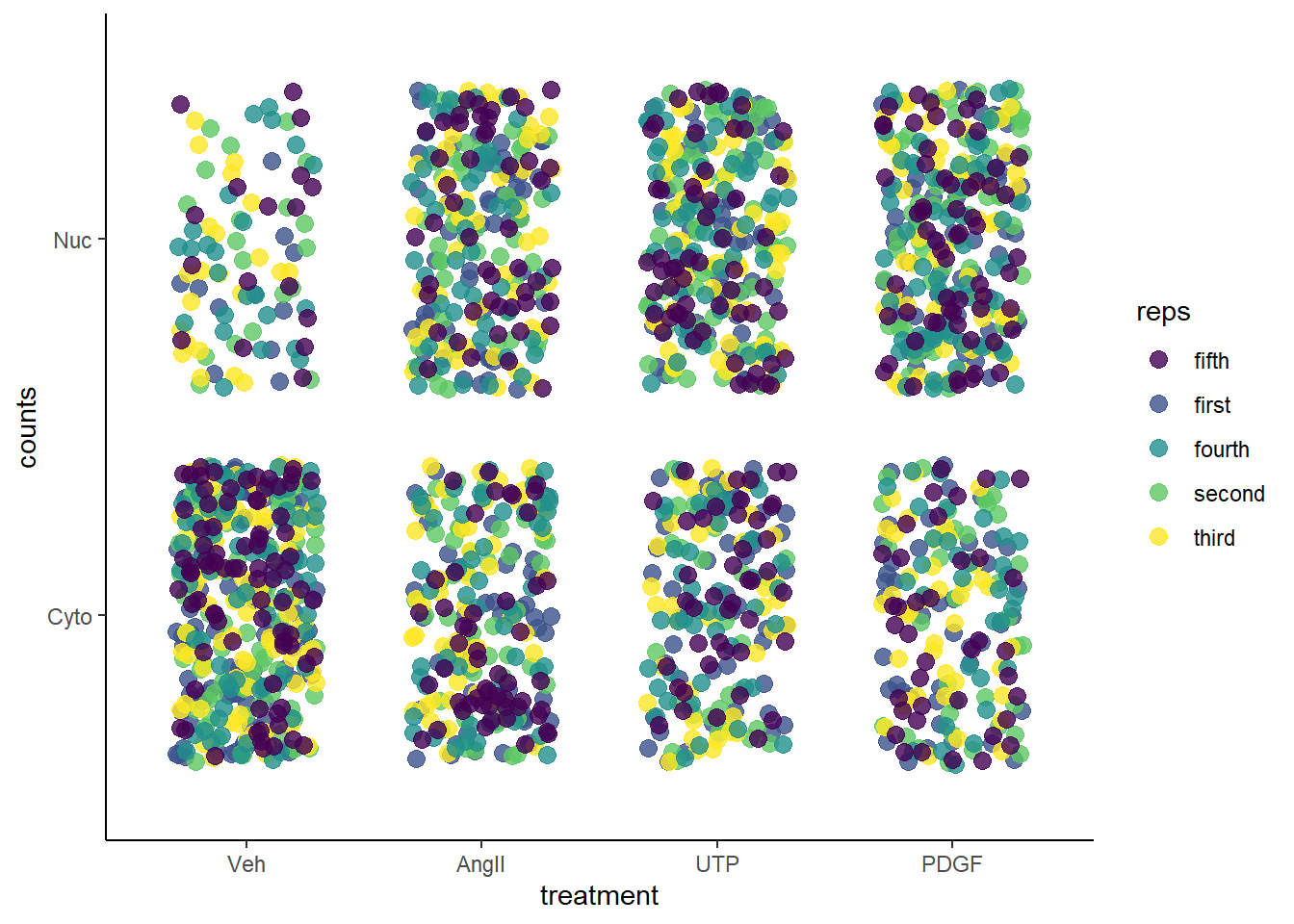 ## Linear model
Since these are discrete nominal counts the data are expect to fit a binomial distribution. Thus, the binomial family is chosen for the generalized linear model.
Within each replicate every cell scored under the different exposure conditions are clearly not independent from every other cell. The cell culture conditions are highly homogenous within each plate and between the different plates on any given day. They were measured on cultured cells of the same passage date and involve the use of a common source of reagents. All intracellular localization counts within each replicate are intrinsically-related. This is a scientific, not a statistical, judgement.
In the smnfat data set, reps is a grouping variable indicating the replicate id. Adding (1|reps) to the model accounts for this, assuring that a random intercept will be calculated for each replicate. See Table 2 in the lme4 vignette for more information.
Finally, because we want to compare all levels of the predictor groups to each other, we’re using the offset key 0+. Here, the model will report fixed coefficient values for each level of the variable, rather than values that are in reference to a common intercept. This provides a logit score for each of the 4 stimuli.
The regression output has a lot of information, but we’re only going to compare the coefficient values for the different levels of treatment:
model2 <- glmer(counts~0+treatment + (1 | reps), family = binomial, data)
summary(model2)
## Generalized linear mixed model fit by maximum likelihood (Laplace
## Approximation) [glmerMod]
## Family: binomial ( logit )
## Formula: counts ~ 0 + treatment + (1 | reps)
## Data: data
##
## AIC BIC logLik deviance df.resid
## 2523.0 2551.0 -1256.5 2513.0 1995
##
## Scaled residuals:
## Min 1Q Median 3Q Max
## -1.3497 -0.9820 -0.4524 0.8350 2.2103
##
## Random effects:
## Groups Name Variance Std.Dev.
## reps (Intercept) 0.01025 0.1012
## Number of obs: 2000, groups: reps, 5
##
## Fixed effects:
## Estimate Std. Error z value Pr(>|z|)
## treatmenta -1.47943 0.12367 -11.963 < 2e-16 ***
## treatmentb -0.03208 0.10036 -0.320 0.749195
## treatmentc 0.36488 0.10168 3.589 0.000332 ***
## treatmentd 0.49077 0.10277 4.776 1.79e-06 ***
## ---
## Signif. codes: 0 '***' 0.001 '**' 0.01 '*' 0.05 '.' 0.1 ' ' 1
##
## Correlation of Fixed Effects:
## tretmnt trtmntb trtmntc
## treatmentb 0.165
## treatmentc 0.163 0.201
## treatmentd 0.161 0.199 0.19646.2.1 Inference
The tests above in the model summary are for the null that the coefficient estimates equal zero. Sometimes that’s a useful test. Here it is not useful, for scientific reasons.
A logit of zero corresponds to a 50:50 proportion of NFAT for the nucleus to cytosol. In fact, given the much lower nuclear to cytosol ratio in unstimulated cells (see the figure), a 50:50 proportion would represent some level of intrinsic activation!
Instead, what we’re interested are group comparisons.
The scientific question driving this experiment is whether the effects of the three mitogens differ from each other, and from the negative control.
The fixed effect coefficient values in the summary output, which are in units of logit, are estimates of the effect sizes for each level of treatment.
The question is, how to compare these effect size values?
We can do so using the same Wald test, but in a way that compares one group to the next. The difference between two coefficient values divided by a standard error gives us the z statistic, which is standard normal distributed.
\[z=\frac{\beta-\beta_0}{SE_\beta}\sim N(0,1)\]
This is a multiple comparison problem, basically identical to the multiple comparison problem we see after an ANOVA when we wish to compare many group means. Here, we want to compare logit values.
Fortunately, packages have been devised for this purpose when dealing with linear model objects.
The multcomp package offers the glht function with which to run these tests. In regression jargon, we specify the contrasts of interests (meaning, we tell it what coefficient comparisons we want made). Recall the Tukey HSD? You pull it out when you wish to make all possible comparisons. That’s done below.
model3 <- summary(glht(model2, linfct=mcp(treatment="Tukey")))
summary(model3)
##
## Simultaneous Tests for General Linear Hypotheses
##
## Multiple Comparisons of Means: Tukey Contrasts
##
##
## Fit: glmer(formula = counts ~ 0 + treatment + (1 | reps), data = data,
## family = binomial)
##
## Linear Hypotheses:
## Estimate Std. Error z value Pr(>|z|)
## b - a == 0 1.4473 0.1458 9.925 <0.001 ***
## c - a == 0 1.8443 0.1468 12.566 <0.001 ***
## d - a == 0 1.9702 0.1475 13.354 <0.001 ***
## c - b == 0 0.3970 0.1277 3.108 0.0103 *
## d - b == 0 0.5229 0.1286 4.066 <0.001 ***
## d - c == 0 0.1259 0.1296 0.971 0.7649
## ---
## Signif. codes: 0 '***' 0.001 '**' 0.01 '*' 0.05 '.' 0.1 ' ' 1
## (Adjusted p values reported -- single-step method)Recall that a=Veh, b=AngII, c=UTP and d=PDGF.
Thus, only UTP and PDGF responses are equivalent. All other comparisons show a differential response. Each mitogen induces nuclear translocation relative to veh. And both UTP and PDGF differ from AngII in the level of response they evoke.
You’ll note that the p-values are adjusted for multiple comparisons.
46.3 Alternative analysis
What researchers commonly do with data like these is to calculate proportions and run t-tests on same.
This script munges the proportions out of the original count data, ultimately yielding the mean and SD for the replicates within each treatment level.
group_by(data, reps, treatment) %>%
  summarise(prop=sum(counts)/100) %>%
  group_by(treatment) %>%
  summarise(mean=mean(prop),
            se=sd(prop)/sqrt(5)
            )
## `summarise()` has grouped output by 'reps'. You can override using the `.groups` argument.## # A tibble: 4 x 3
## treatment mean se
## <chr> <dbl> <dbl>
## 1 a 0.186 0.0225
## 2 b 0.492 0.00860
## 3 c 0.59 0.0352
## 4 d 0.62 0.0207The script calculates the estimates for the proportion sizes from the logit coefficient estimates produced through linear modeling. You can see they are in almost perfect agreement. That’s because MLE is
#calculate mean in prob units from logit units
coef <- summary(model2)$coefficients[,1]
round(exp(coef)/(exp(coef)+1), 3)
## treatmenta treatmentb treatmentc treatmentd
## 0.186 0.492 0.590 0.620However, you can see that the SE estimates for each of the coefficients derived by logistic regression are quite different from the SE’s that would become part of the t-test calculation.
#calculate SE in prob units from logit units
coef2 <- summary(model2)$coefficients[,2]
exp(coef2)/(exp(coef2)+1)
## treatmenta treatmentb treatmentc treatmentd
## 0.5308775 0.5250684 0.5253974 0.5256687Here’s the main problem I have t-testing proportions (as opposed to Wald testing): Proportions don’t have anything that remotely resembles a Gaussian distribution. Proportions have limits at the lower (0) and upper (1) values. Gaussian distributions are limitless. Binomial distributions are skewed. Gaussian distributions are symmetrical.
The t-test should be reserved for variables that have a Gaussian distribution.