Chapter 6 Stats: The Big Picture

To call in the statistician after the experiment is done may be no more than asking him to perform a post-mortem examination: he may be able to say what the experiment died of. ~ Sir Ronald Aylmer Fisher

library(tidyverse)
library(Hmisc)

Let’s start by listing out some key characteristics that most biomedical experiments share in common.

They…

tend to involve the use of relatively small sample sizes.
are usually highly exploratory in nature, measuring new variables under new conditions.
generate data that are either counted as discrete counts or measurements of continuous scalars.
are structured as a small group of fairly common experimental designs.
are usually interpreted in a binary way; as having “worked,” or not.
test hypotheses (though too often these are unstated).
aspire for rigor, replicability and reproducibility.
aspire to be unbiased.

The stakes of our work can be pretty high. These include the higher ideals such as the validation of novel scientific paradigms, the steady advancement of knowledge, and opening the door to impact, particularly in the realm of human diseases and suffering.

But no less motivating are the issues more related to the professional practice of science. These include ego, the completely natural impulse to seek out validation for an idea, publication and/or commercialization, time to degree, career viability, scientific reputations, and coveted research/investment funds.

The point is that the process of scientific discovery is driven both by ideals and by biases. This is nothing new. What may be new is the fact that you are not shielded from bias simply because you work in a university and your work is peer-reviewed.

The one big concept that I hope you embrace is that the statistical design and analysis of experiments serves antibias framework. A biomedical researcher operates within that framework to conduct reasonably unbiased work.

The statistical approaches covered in this course, it turns out, were invented long ago with this purpose in mind.

6.1 What are experimental statistics?

Experimental statistics are used

in experimental planning,
to summarize data into simpler descriptive models,
as procedures to make valid inferences,
to serve as framework for conducting unbiased research.

Chances are that you thought biostats was only applied math or that part of software used to produce summaries and p-values after a trove of data has been collected. It is much more than that.

6.1.1 Descriptive modeling

Statistical models are ways of simplifying or summarizing data so that they can be more readily described and interpreted.

For example, if we have a sample in which blood glucose levels are measured in each of many subjects, clarity demands we explain those results in terms of summary statistics. Thus, we use parameters like the sample mean and standard deviation, or median and ranges or percentiles to describe what we’ve just measured.

The alternative is unthinkable today (but common long ago), which is to discuss each replicate individually.

Descriptive modeling is just summarizing what we found in a sample and extending that to the population that was just sampled.

To emphasize that sample parameters differ from population parameters, the standard in statistical notation is to use roman characters to indicate samples and greek characters to indicate the population. For example,

parameter	sample	population
mean	\(\bar y\)	\(\mu\)
standard deviation	\(s\)	\(\sigma\)
variance	\(s^2\)	\(\sigma^2\)

Thus, the sample mean, \(\bar y\) is an estimate of the population mean, \(\mu\).

Statistical tests also have a descriptive element in that they convey information about the experimental design. If you say, “I’m working up a two-tailed paired t-test,” say no more.

From that alone I know something about your hypothesis, how your replicates are handled, the number of predictor groups, and the type of data you’re measuring.

Regression models also describe data. For example, here is the well-known Michaelis-Menten model that describes product formation as a function of substrate concentration.
\[[P]=\frac{[S][Vmax]}{[S]+Km}\]

That’s a model we might fit to certain kinds of enzyme kinetic data. The model is used to estimate scientifically meaningful parameters, like \(V_{max}\) and \(K_m\), from experiments where we control \([S]\) while measuring \([P]\).

In fact, mathematical statistics is actually just modeling. And modeling is the process of simplifying experimental data into something more coherent.

Take a simple example of two groups shown here. Each group has been fit to a simple, very common model: sample mean and standard deviation.

Clearly, that model fits the control group much better than it fits the treatment group.

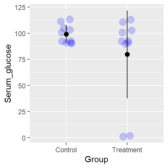
Figure 6.1: Is the mean for each these groups a good descriptive model?

Why do I say that? The treatment group data are much more skewed. Most of the data values are greater than the mean of the group. Sure, a mean can be calculated for that group, but it serves as a fairly crappy summary. Perhaps some other model (or group of statistical parameters) would better convey how these data behave?

This is to point out that learning statistics is about learning to make judgments about which models are best for describing a given data set.

6.1.2 Statistical inference

There are two main types of inference researchers make.

One type is to infer whether an experiment “worked” or not…the so-called “significance test.”

This familiar process involves calculating a test statistic from the data (eg, t-test, F-tests, etc) and then applying a threshold rule to its value. If the test passes the rule, we conclude the experiment worked. I cover this type of inference in much more detail in the p-value chapter 13. We’ll talk about this one over and again throughout the course.

A second type of inference is to use a sample parameters as estimates for values of the variable within the sampled population. For example, the average height students in an Emory graduate biostats course can be used as an estimate of all biostats students (or all Emory graduate students).

Both descriptive and statistical inference are subject to error. By random chance/luck-of-the-draw our sample estimates can be off the mark. Usually, we don’t how wrong we might be.

A great example for this is seeing the various

The real difficulty with inference is we can never know for certain whether we are right or wrong.

They are called random variables for a reason. It pays to have a very healthy respect for the role played by random chance in determining the values of our parameter estimates. If we were to completely redo a fully replicated experiment once more, we would almost certainly arrive at different numbers. In a well behaved system, they’d likely be in the same ballpark as those of the first experiment. But they would still differ.

To illustrate, copy and paste the code chunk below. It replicates a random triplicate sample six times, taking six means. Unlike in real life, the population parameters are known (because I coded them in): \(\mu=2\) and \(\sigma=0.4\). You can run that chunk tens of thousands of times and never get a “sample” with one mean that has a value of exactly 2, even though that’s the true mean of the population that was sampled.

x <- replicate(6, rnorm(3, 2, 0.4))
apply(x, 2, mean)

## [1] 2.092121 2.025281 2.093270 1.612758 2.096955 2.276354

6.1.3 Experimental design

Experimental planning that involves dealing with statistical issues is referred here as experimental design.

This involves stating a testable statistical hypothesis and establishing a series of decision rules in advance of data collection. These rules range from subject selection and arrangement, predetermination of sample size using a priori power analysis, setting some data exclusion criteria, defining error tolerance, specifying how the data will be transformed and analyzed, declaring a primary outcome, on up to what statistical analysis will be performed on the data.

Experimental design is very common in prospective clinical research. Unfortunately, very few basic biomedical scientists practice anything remotely like this.

Most biomedical researchers begin experiments with only vague ideas about the statistical analysis, which is usually settled on after the fact. Much of the published work today is therefore retrospective, rather than prospective. Yet, most researchers tend to use statistics that are largely intended for prospective designs. That’s a problem.

6.1.4 Statistics as an anti-bias framework

If you are ever asked (for example, in an examination) what purpose is served by a given statistical procedure, and you’re not exactly sure, you would be wise to simply offer that it exists to prevent bias. That may not be the answer the grader was hunting for, but it is almost surely correct.

The main purpose of “doing” statistical design and analysis of experiments is to control for bias. Humans are intrinsically prone to bias and scientists are as human as anybody else. Holding or working on a PhD degree doesn’t provide us a magic woo-woo cloak to protect us from our biases.

Therefore, whether we choose to admit it or not, bias infects everything we do as scientists. This happens in subtle and in not so subtle ways. We work hard on our brilliant ideas and, sometimes, desperately wishing to see them realized, we open the door to all manner of bias.

Here are some of the more important biases.

6.1.4.1 Cognitive biases

From a statistical point of view biases can be classified into two major groupings. The first are Cognitive biases. These are how we think (or fail to think) about our experiments and our data.

These frequently cause us to make assumptions that we would not if we only knew better or were wired differently. Following a negative result, if you ever find yourself declaring, “how could this not work!?!” you are in the throes of a pretty deep cognitive bias. In bench research, cognitive biases can prevent us from building adequate controls into experiments or lead us to fail to think about alternative explanations for results, or prevent us from spotting confounding variables or recognizing telling glitches in the data as meaningful. Cognitive biases are the rose-tinted glasses worn by all scientists.

6.1.4.2 Systematic biases

The second genaral bias are systematic biases. Systematic biases are inherent to our experimental protocols, the equipment and materials we use, the timing and order by which tasks are done, the subjects we select and, yes (metaphorically), even whether the data are collected left-handed or right-handed, and how data is handled or transformed.

Systematic biases can yield the full gamut of unintended outcomes, ranging between nuisance artifacts to false negatives or positives. For example, poorly calibrated equipment will bias data towards taking inaccurate values. Working forever on an observed phenomenon using only one strain of mouse or cell line may blind us from realizing it might be a phenomenon that only occurs in that strain of mouse or cell line.

6.1.4.3 Scientific misconduct

More malicious biases exist, too. These include forbidden practices such as data fabrication and falsification. This is obviously a problem of integrity. Very few scientists working today are immune from the high stakes issues that pose threats to our sense of integrity.

In the big picture, particularly for the biomedical PhD student, I like to call bias the event horizon of rabbit holes. A rabbit hole is that place in a scientific career where it is easy to get lost for a long, long time. You want to avoid them.

The application of statistical principles to experimental design provides some structure to avoid making many of the mistakes that are associated with these biases. Following a well-considered, statistically designed protocol enforces some integrity onto the process of experimentation. Most scientists find a statistical framework quite livable.

If you give it some thought, the only thing worse than a negative result from a statistically rigorous experiment is a negative result from a statistically weak experiment. With the former at least you know you’ve given it your best shot. That is hard to conclude when the latter occurs.

6.1.4.4 Statistical bias

In statistical jargon something that is said to be biased is inaccurate. Bias, as a statistical term, is a synonym for inaccurate.