Chapter 29 The F distribution
library(tidyverse)29.1 Background
George Snedecor once said that Student’s t distribution is the “distribution that revolutionized the statistics of small samples.” As the inventor of the F distribution, nobody would have faulted Snedecor for praising himself the same way.
The F distribution is heavily used in parametric statistics.
The most common use of the F statistic is to examine ratios for two estimators of population variance. In particular, F-tests in ANOVA are ratios of model variances, at given degrees of freedom, to residual variances, a some other given degrees of freedom. Another common use is to F-test nested regression models to determine if the more complex model provides a better fit for the data.
When the value of this ratio is extreme, the variances are not equivalent, meaning the variance in an experiment is better explained by factor effects than by residual error.
An F distribution represents the null probability distribution for such ratios and is therefore used to test hypotheses involving variances.
F is used widely in statistics to answer a simple question: Are two samples drawn from populations that have the same variance? For example, the F statistic serves as an omnibus test for ANOVA, and is used in regression to determine which of two models best fit a dataset, and is also used for normality tests.
More generally, the F statistic can be used to analyze a proportion of two random, \(\chi^2\)-distributed variables.
29.1.1 Sample Variance and F’s PDF
A sample of size \(i=n\) for a random, independent variable \(X\) can take on the values \(x_1, x_2,...x_i\). The sample mean is \(\bar x=\frac{1}{n}\sum\limits_{i=1}^{n}x_i\) with \(df=n-1\) degrees of freedom.
The sum of the residual deviation from the sample mean, also known as the sample “sum of squares,” (\(SS\)) is: \[SS=\sum\limits_{i=1}^{n}(x_i-\bar x)^2\]
The sample variance is: \[s^2=\frac{\sum\limits_{i=1}^{n}(x_i-\bar x)^2}{df}\]
The sample variance is otherwise known as the “mean square” in jargon commonly associated with ANOVA: \[MS=\frac{\sum\limits_{i=1}^{n}(x_i-\bar x)^2}{df}\]
The \(MS_{df}\) of a normally distributed random variable \(X\) with \(df\) will have a \(\chi^2_{df}\) distribution.
Now let the normally distributed variables \(X1\) and \(X2\) have \(df_1\) and \(df_2\) degrees of freedom, and also variances of \(MS_{df1}\) and \(MS_{df2}\), respectively. The F statistic is:
\[F=\frac{MS_{df1}}{MS_{df2}}\]
The probability density function for the F statistic is: \[f(x)=\frac{(\frac{df_1}{df_2})^\frac{df_1}{2}\Gamma[\frac{(df_1+df_2)}{2}]x^{\frac{df_1}{2}-1}}{\Gamma[\frac{df_1}{2}]\Gamma[\frac{df_2}{2}][1+(\frac{df_1x}{df_2})]^{\frac{(df_1+df_2)}{2}}}\]
29.2 df
R’s function for the F PDF is df and returns a value for the probability of F, given its degrees of freedom. It takes as arguments a value for x, which represents F. x can either be unique value or represent a range of values. Other arguments include df1 and df2, which represent values for the degrees of freedom represented in the numerator and denominator, respectively.
There is a unique F distribution for any combination of df1 and df2.
The exact probability when F has a value of 2.5 and 2 and 10 degrees of freedom (\(F_{df_1,df_2=2.5}\)) is:
df(2.5, df1=2, df2=10)## [1] 0.0877915The distribution of the F statistic can vary quite markedly depending upon the combination of df1 and df2.
For example, let’s imagine the 3 curves below correspond to each of 3 different one-way ANOVA experimental designs. The red distribution represents a null distribution for F for an ANOVA experiment having 3 predictor groups with a sample size of 5 independent subjects per group. The blue distribution represents the null of F for an experiment of 10 groups with 3 replicates per group. The green distribution is the null of F for an experiment with 20 groups, each with 4 replicates.
Thus, since the numerator and denominator of the F statistic represent two different populations, the F distribution is extraordinarily flexible in terms of the comparisons that can be made using it!
ggplot(data.frame(x=c(0,6)), aes(x)) +
  stat_function(fun="df", args=list(df1=2, df2=12), color="red")+
  stat_function(fun="df", args=list(df1=9, df2=20), color="blue") +
  stat_function(fun="df", args=list(df1=19, df2=60), color="green")+
  labs(x ="F", y="p(F)")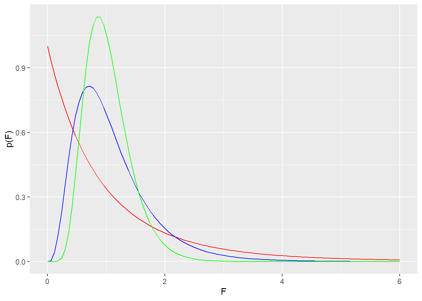
29.3 pf
The cumulative distribution function for F returns the cumulative probability under the F distribution for a value of the F statistic and a given pair of degrees of freedom.
pf(q=4, df1=2, df2=12)## [1] 0.953344A p-value is returned by using the following argument: lower.tail=F. Thus, the probability of an F statistic whose value is 4.0 or larger is:
pf(q=4, df1=2, df2=12, lower.tail=F)## [1] 0.046656ggplot(data.frame(x=c(0,6)), aes(x)) +
stat_function(fun="pf", args=list(df1=2, df2=12), color="red")+
stat_function(fun="pf", args=list(df1=9, df2=20), color="blue") +
stat_function(fun="pf", args=list(df1=19, df2=40), color="green")+
labs(x ="F", y="p(F)")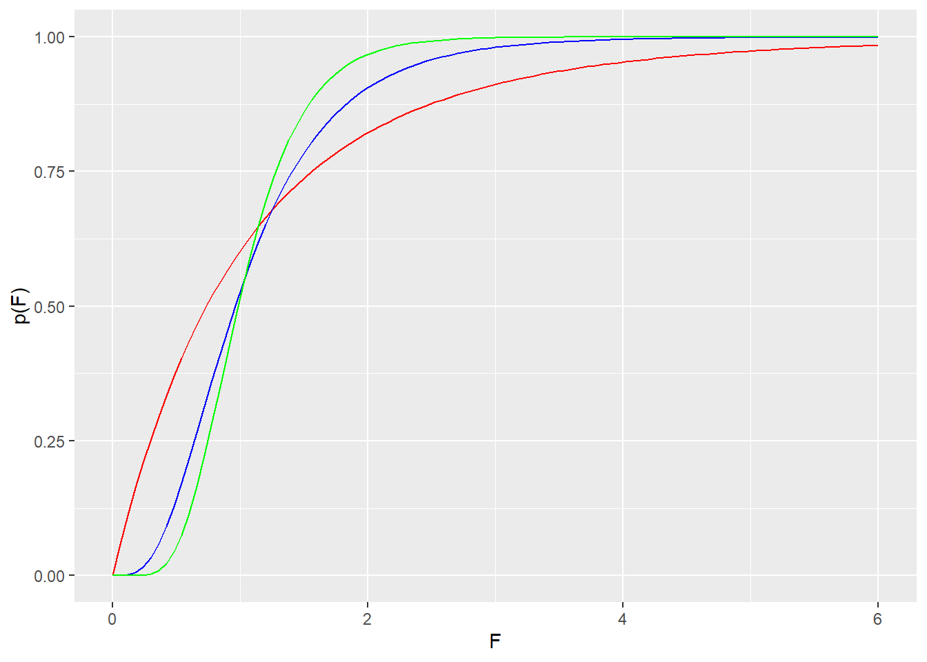
29.4 qf
The inverse cumulative probability function for the F distribution is qf. This function will take a probability as an argument, and return the corresponding value of the F statistic for a given pair of degrees of freedom.
qf(p=0.95, df1=2, df2=12)## [1] 3.885294An F statistic limit for a given p-value can be calcuated using the lower.tail=F argument.
qf(p=0.05, df1=2, df2=12, lower.tail=F)## [1] 3.885294ggplot(data.frame(x=c(0,1)), aes(x)) +
stat_function(fun="qf", args=list(df1=2, df2=12), color="red")+
stat_function(fun="qf", args=list(df1=9, df2=20), color="blue") +
stat_function(fun="qf", args=list(df1=19, df2=40), color="green")+
labs(x ="p(F)", y="F")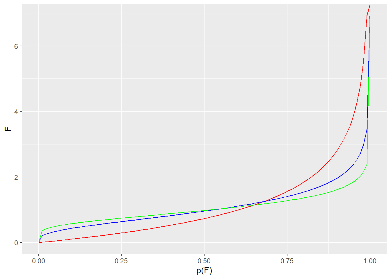
29.5 rf
The rf function can be used to generate n random F statistic values for a given pair of degrees of freedom.
rf(n=10, df1=2, df2=12)## [1] 0.5597275 0.9402234 0.5752848 1.8002392 0.6221102 0.2859954 1.4767106
## [8] 2.2144931 1.4721874 2.4914325