Chapter 14 Reproducible Data Munging in R
library(datapasta)
library(tidyverse)
library(cowplot)
library(viridis)
Data munging is the process of taking data from one source(s) and working it into a condition where it can be analyzed. Every data set will differ and so every data munge will be custom.
Data munging is a bit like organic chemistry. We know what we want to create. We know the starting materials that we have on hand. We work work with reactions and intermediates necessary to produce that final product.
Here is one example of the munging process. The exercise converts an excel file data source into a format that can be used in R.
The data source is formatted in such a way that reading the file is buggy, and not pragmatic. We will use the import function (datapasta) and a handful of functions in the tidyverse package to get it into R and into a long table tidy format.
Note especially how every transaction with the data is recorded. Anyone who has this source data file can start with the same excel file and get an identical outcome. That’s reproducibility.
14.1 Jaxwest7 data
The Jaxwest7 data set is a Jackson Labs experiment conducted using an obese mouse model of diabetes type 2. The experiment tests whether a drug used to treat type2 diabetes, rosiglitazone, is effective in the model.
From the protocol, half the subjects receive the antidiabetic drug, the other receive vehicle as placebo. The syndrome is assessed by measuring two response variables: body weight and blood glucose concentrations. There are two explanatory variables: day of study and drug treatment.
The experimental design is therefore multivariate (weight, blood glucose) two-factor (drug treatment, day) ANOVA with repeated measures on the day variable.
Our ultimate goal is to create a dataset for MANOVA analysis.
The purpose of this chapter, for now, is to illustrate how to retrieve and process data to prepare it for analysis. We will use datapasta to copy the data from the spreadsheet into code, which illustrates the Addin feature of RStudio.
14.1.1 Inspect the source data
Download the Jaxwest7.xls file from the mouse phenome database to your machine and open it with spreadsheet software such as Excel.
First go to the BloodGlucoseGroups tab.
This is readable file, but complex. In fact, this sheet illustrates what unstructured data looks like.
- Almost every column has cells containing multiple types of values.
- The first 8 rows have various descriptor text, including a logo.
- Rows 9-14 have some other definitions.
- Scroll way over to the right and some graphs pop up.
- The data we are interested in are in rows 15 to 42, and in columns F to S. Each of those columns has two column names, a date and a day. A variable column should have only one name.
Additionally…
Columns T and U have several missing values, because those animals were used for autopsy. We’re going to have to ignore their response values.
Cell F21 is a character value indicative of an out-of-range test result.
Columns 43 to 146 are missing entirely. Below the array are some summary statistics, each of which is a different parameter.
Finally, cage and mouse ID’s are not recorded.
Now go to the BodyWeightsGroups tab.
The structural issues are about the same as for the BloodGlucoseGroups sheet. Here there are cage ID’s but no mouse ID’s.
Most notably, there are only 7 rows of body weights in the rosiglitazone treatment group, whereas there are 8 rows in the corresponding glucose group.
These are not a spreadsheets that can be imported whole scale directly into R with ease. Instead, we need to grab only the data we need. Then we’ll use R to structure it for analysis.
14.2 Munge the glucose data into R
Let’s start with the glucose data R. The goal is to create a dataframe object with the following variables: animal id, day, treatment, and glucose value.
Glucose concentrations were measured twice per day on odd-numbered days plus day 12. Each column represents a blood draw session. This was done on each of 16 animals. Half were in a placebo group, half were in a drug group.
We’ll omit day 15 due to the NA values (those mice were harvested for autopsy, and so day 15 breaks the time series).
We’ll also omit the last row in the rosiglitazone group because it doesn’t have a corresponding match in the body weight data.
We assume each row represents a unique mouse and that the rows in the glucose and body weight data correspond. This is tenuous and not ideal.
14.2.0.1 Step 1
Deal with cell F21. It’s value in the excel spreadsheet is “Hi,” a character value rather than a numeric. We have two options: Assign it an NA value, or impute.
Since this is a related-measures time series with multiple other glucose measurements for that specific replicate, we’ll impute by using the average of all these other measurements.
Calculate the value that will be imputed:
#Use datapasta to paste in vector values. Calculate their mean. Then impute value for cell F21 in original data set by exchanging the value "Hi" with the mean produced here.
F21 <- mean(c(449L, 525L, 419L, 437L, 476L, 525L, 499L, 516L, 485L, 472L, 535L, 500L, 497L)
); F21
## [1] 487.3077Ideally, you’d import the data with the “Hi” value and fix it in R, to have a contiguous reproducible record for the imputation. In this case, I’m getting some anomalies using read_excel from readr, which seem related to the spreadsheet formatting. Leaving “Hi” in F21 causes some another issue with the datapasta importer that require additional not-fun munging. So it will be fixed in situ.
14.2.0.2 Step 2
Fix the F21 cell in the spreadsheet file by imputing the value from above.
14.2.0.3 Step 3
Copy the spreadsheet array F15:S41 to the clipboard. This is 14 columns and 15 rows of glucose data. All values are numeric and represent the same variable: blood glucose concentration.
This omits the last replicate from the rosiglitazone glucose group. This is due to the fact that the body weight data only are for four rosiglitazone animals.
Use the datapasta package Addin for this procedure. Create an object name, put the cursor next to it, and select Paste as Tribble from the Addins drop down menu. You’ll find the Addins drop down just below the RStudio main menu.
jw7gluc <- tibble::tribble(
             ~V1, ~V2, ~V3, ~V4, ~V5, ~V6, ~V7, ~V8, ~V9, ~V10, ~V11, ~V12, ~V13, ~V14,
             136, 270, 162, 165, 192, 397, 172, 148, 291,  239,  192,  172,  235,  153,
             345, 518, 429, 413, 456, 487, 468, 419, 507,  559,  420,  415,  511,  464,
             190, 301, 311, 361, 398, 465, 388, 392, 453,  421,  355,  381,  394,  444,
             434, 504, 453, 392, 350, 400, 458, 387, 342,  368,  355,  429,  373,  501,
             424, 486, 447, 417, 496, 484, 468, 423, 472,  507,  458,  456,  519,  570,
             170, 208, 134, 129, 147, 141, 241, 128, 162,  163,  222,  438,  307,  252,
             487, 449, 525, 419, 437, 476, 525, 499, 516,  485,  472,  535,  500,  497,
             218, 273, 254, 265, 338, 386, 287, 236, 347,  235,  432,  450,  509,  326,
             179, 184, 124, 107, 108, 149, 142, 143, 112,  233,  113,  137,  106,  150,
             260, 381, 174, 140, 132, 138, 164, 137, 122,  140,  102,  174,  120,  135,
             115, 191, 132, 132, 169, 158, 129, 120, 122,  157,   94,  141,  120,  166,
             526, 517, 465, 394, 310, 269, 213, 185, 145,  201,  131,  258,  114,  160,
             325, 252, 203, 158, 135, 162, 164, 181, 150,  177,  162,  192,  170,  162,
             329, 296, 212, 159, 156, 200, 139, 143, 164,  150,  119,  193,  148,  188,
             230, 414, 408, 179, 432, 288, 163, 240, 185,  208,  138,  208,  153,  140
             )
Notice how R coerces unique variable names for each column. That’s fine, but we’ll need to fix them.
14.2.0.4 Step 4
Convert from a wide to a long format, and check.
gluc <- jw7gluc %>% pivot_longer(cols=V1:V14,
                              names_to = "V",
                              values_to="glucose")
gluc
## # A tibble: 210 x 2
## V glucose
## <chr> <dbl>
## 1 V1 136
## 2 V2 270
## 3 V3 162
## 4 V4 165
## 5 V5 192
## 6 V6 397
## 7 V7 172
## 8 V8 148
## 9 V9 291
## 10 V10 239
## # ... with 200 more rows14.2.0.5 Step 5
Create variables for ID, day, blood draw and treatment.
  id <- rep(LETTERS[1:15], each=14)
  day <- rep(rep(c(1, 3, 5, 7, 9, 11, 12), each=2), 15)
  draw <- rep(rep(c("early", "late"), 7),15)
  treat <- c(rep("placebo", 8*14 ), rep("rosiglitazone", 7*14))
14.2.0.6 Step 6
Add the variables to the long data frame while removing the irrelevant “V” variable.
gluc <- add_column(gluc,
                   id,
                   day,
                   draw,
                   treat,
                   .before=T) %>%
  select(-one_of("V"))
gluc
## # A tibble: 210 x 5
## id day draw treat glucose
## <chr> <dbl> <chr> <chr> <dbl>
## 1 A 1 early placebo 136
## 2 A 1 late placebo 270
## 3 A 3 early placebo 162
## 4 A 3 late placebo 165
## 5 A 5 early placebo 192
## 6 A 5 late placebo 397
## 7 A 7 early placebo 172
## 8 A 7 late placebo 148
## 9 A 9 early placebo 291
## 10 A 9 late placebo 239
## # ... with 200 more rows14.2.0.7 Step 7
Convert every variable except for glucose to a factor.
  cols <- c("id", "day", "draw", "treat")
gluc[cols] <- lapply(gluc[cols], factor)
gluc
## # A tibble: 210 x 5
## id day draw treat glucose
## <fct> <fct> <fct> <fct> <dbl>
## 1 A 1 early placebo 136
## 2 A 1 late placebo 270
## 3 A 3 early placebo 162
## 4 A 3 late placebo 165
## 5 A 5 early placebo 192
## 6 A 5 late placebo 397
## 7 A 7 early placebo 172
## 8 A 7 late placebo 148
## 9 A 9 early placebo 291
## 10 A 9 late placebo 239
## # ... with 200 more rows14.2.0.8 Step 8
Average the early and late blood draws, to get one glucose value per day.
gluc <- gluc %>%
  group_by(id, day, treat) %>%
  summarise(glucose=mean(glucose))
## `summarise()` has grouped output by 'id', 'day'. You can override using the `.groups` argument.gluc## # A tibble: 105 x 4
## # Groups: id, day [105]
## id day treat glucose
## <fct> <fct> <fct> <dbl>
## 1 A 1 placebo 203
## 2 A 3 placebo 164.
## 3 A 5 placebo 294.
## 4 A 7 placebo 160
## 5 A 9 placebo 265
## 6 A 11 placebo 182
## 7 A 12 placebo 194
## 8 B 1 placebo 432.
## 9 B 3 placebo 421
## 10 B 5 placebo 472.
## # ... with 95 more rows14.2.0.9 Step 9
Now here’s a summary of all the replicate values in tabular form.
gluc %>%
  group_by(day, treat) %>%
  summarise(
    n=length(glucose),
    mean=round(mean(glucose)),
    sd=round(sd(glucose)),
    sem=round(sd/sqrt(n)),
    min=round(min(glucose)),
    max=round(max(glucose))
  )
## `summarise()` has grouped output by 'day'. You can override using the `.groups` argument.## # A tibble: 14 x 8
## # Groups: day [7]
## day treat n mean sd sem min max
## <fct> <fct> <int> <dbl> <dbl> <dbl> <dbl> <dbl>
## 1 1 placebo 8 338 128 45 189 469
## 2 1 rosiglitazone 7 300 120 45 153 522
## 3 3 placebo 8 330 131 46 132 472
## 4 3 rosiglitazone 7 213 111 42 116 430
## 5 5 placebo 8 378 115 41 144 490
## 6 5 rosiglitazone 7 200 89 34 128 360
## 7 7 placebo 8 352 132 47 160 512
## 8 7 rosiglitazone 7 162 30 11 124 202
## 9 9 placebo 8 379 132 47 162 533
## 10 9 rosiglitazone 7 162 22 8 131 196
## 11 11 placebo 8 386 99 35 182 504
## 12 11 rosiglitazone 7 154 29 11 118 194
## 13 12 placebo 8 410 117 41 194 544
## 14 12 rosiglitazone 7 145 17 6 128 168Woot! We’ll visualize at the end.
14.3 Munge the bodyweight data
The goal here is to create a data frame of the body weight data that is symmetric to the glucose dataframe created above. That’s because the ultimate goal is to join the two together into a single dataframe.
The major difference between the two sheets in the excel file is the body weights are measured daily rather than every other day as for glucose. We’ll therefore toss out some data. Sad.
14.3.0.1 Step 1
From the BodyWeightsGroups sheet we copy cells F15:T45 to the clipboard. Name an object in the code junk. Then on the Addins drop down menu select Paste as tribble
jw7bw <- tibble::tribble(
  ~V1,  ~V2,  ~V3,  ~V4,  ~V5,  ~V6,  ~V7,  ~V8,  ~V9, ~V10, ~V11, ~V12, ~V13, ~V14, ~V15,
  31.9, 32.1, 32.8,   33, 33.3, 33.2, 33.2, 32.8, 33.5,   34, 34.2, 34.9, 35.2, 35.8, 36.1,
  38.1, 38.4, 38.7, 38.5, 38.8, 38.8, 38.9, 38.6, 39.4, 39.4,   39, 39.4, 39.7, 39.3, 39.1,
  31, 31.7, 31.9,   32, 32.9, 33.1, 33.5, 33.6, 34.3, 34.4, 34.7, 35.5, 35.4, 35.5, 35.4,
  36.4, 35.9, 36.8, 36.9, 37.3, 37.1, 37.4, 37.4, 36.8, 37.4, 37.1,   38, 37.4,   38, 37.9,
  38.9, 38.5, 39.2, 39.1, 39.8, 39.3, 39.3, 39.5, 39.7, 40.1, 40.3,   41, 40.9, 41.4, 41.4,
  33.8, 34.2, 34.2, 33.9, 34.7,   35, 35.3, 35.3, 35.8, 36.1, 36.7, 37.3, 37.5, 38.4, 38.7,
  34.6,   35,   35, 35.1, 35.6, 35.5, 35.7, 36.1, 35.9, 35.9, 35.5, 35.3, 35.2,   35, 34.6,
  33.4, 33.6, 34.2, 33.8, 34.3, 34.6, 34.7, 34.9, 34.9, 35.4, 35.6, 35.8, 36.1, 35.9, 35.8,
  31.9, 31.9, 32.6, 33.2, 34.3, 34.7, 35.3, 35.1, 35.4, 35.6,   36, 36.9,   37, 38.7, 38.8,
  33.4, 34.1, 35.2, 35.8, 36.7, 37.4, 38.2, 38.7, 39.5, 40.1, 40.2, 40.6,   41, 41.7,   42,
  32.8, 33.7, 34.5, 34.9, 35.5,   36,   36, 36.2,   36, 36.9, 36.9, 37.6, 38.1, 39.2, 39.5,
  37.9, 38.8, 39.9, 40.4, 41.5, 42.5, 43.3, 43.8, 44.5, 44.7, 45.1, 45.7, 46.3, 47.1, 47.1,
  35.9, 37.2,   38, 38.6, 39.4,   40, 40.5,   41, 41.2, 42.3, 43.2, 43.9, 44.2, 44.3, 44.9,
  35.2, 36.5, 37.4,   38,   39, 39.5, 40.4, 40.7, 40.9, 41.9, 42.5, 43.5,   44, 44.1, 44.7,
  35.8, 36.6, 37.3, 37.7, 38.4, 38.4, 39.3, 40.1, 40.9, 41.4, 41.7, 42.3, 42.2, 42.9, 43.3
)
14.3.0.2 Step 2
Select only the days that correspond to the glucose measurement days.
bw <- jw7bw %>%
  select(c(V1, V3, V5, V7, V9, V11, V12))
bw
## # A tibble: 15 x 7
## V1 V3 V5 V7 V9 V11 V12
## <dbl> <dbl> <dbl> <dbl> <dbl> <dbl> <dbl>
## 1 31.9 32.8 33.3 33.2 33.5 34.2 34.9
## 2 38.1 38.7 38.8 38.9 39.4 39 39.4
## 3 31 31.9 32.9 33.5 34.3 34.7 35.5
## 4 36.4 36.8 37.3 37.4 36.8 37.1 38
## 5 38.9 39.2 39.8 39.3 39.7 40.3 41
## 6 33.8 34.2 34.7 35.3 35.8 36.7 37.3
## 7 34.6 35 35.6 35.7 35.9 35.5 35.3
## 8 33.4 34.2 34.3 34.7 34.9 35.6 35.8
## 9 31.9 32.6 34.3 35.3 35.4 36 36.9
## 10 33.4 35.2 36.7 38.2 39.5 40.2 40.6
## 11 32.8 34.5 35.5 36 36 36.9 37.6
## 12 37.9 39.9 41.5 43.3 44.5 45.1 45.7
## 13 35.9 38 39.4 40.5 41.2 43.2 43.9
## 14 35.2 37.4 39 40.4 40.9 42.5 43.5
## 15 35.8 37.3 38.4 39.3 40.9 41.7 42.314.3.0.3 Step 3
Change from wide to long format and check.
bw <- bw %>% pivot_longer(cols=V1:V12, names_to="V", values_to="weight")
bw
## # A tibble: 105 x 2
## V weight
## <chr> <dbl>
## 1 V1 31.9
## 2 V3 32.8
## 3 V5 33.3
## 4 V7 33.2
## 5 V9 33.5
## 6 V11 34.2
## 7 V12 34.9
## 8 V1 38.1
## 9 V3 38.7
## 10 V5 38.8
## # ... with 95 more rows14.3.0.4 Step 4
Add variables for id, day and treatment.
id <- rep(LETTERS[1:15], each=7)

day <- rep(c(1, 3, 5, 7, 9, 11, 12), 15)

treat <- c(rep("placebo", 8*7), rep("rosiglitazone", 7*7))

bw <- add_column(bw, id, day, treat, .before=T) %>% select(-one_of("V"))
bw
## # A tibble: 105 x 4
## id day treat weight
## <chr> <dbl> <chr> <dbl>
## 1 A 1 placebo 31.9
## 2 A 3 placebo 32.8
## 3 A 5 placebo 33.3
## 4 A 7 placebo 33.2
## 5 A 9 placebo 33.5
## 6 A 11 placebo 34.2
## 7 A 12 placebo 34.9
## 8 B 1 placebo 38.1
## 9 B 3 placebo 38.7
## 10 B 5 placebo 38.8
## # ... with 95 more rows14.3.0.5 Step 5
Factorize each of the variables except for weight.
cols <- c("id", "day", "treat")

bw[cols] <- lapply(bw[cols], factor)
bw
## # A tibble: 105 x 4
## id day treat weight
## <fct> <fct> <fct> <dbl>
## 1 A 1 placebo 31.9
## 2 A 3 placebo 32.8
## 3 A 5 placebo 33.3
## 4 A 7 placebo 33.2
## 5 A 9 placebo 33.5
## 6 A 11 placebo 34.2
## 7 A 12 placebo 34.9
## 8 B 1 placebo 38.1
## 9 B 3 placebo 38.7
## 10 B 5 placebo 38.8
## # ... with 95 more rows14.3.0.6 Step 6
Calculate some descriptive statistics.
bw %>%
  group_by(day, treat) %>%
  summarise(
    n=length(weight),
    mean=mean(weight),
    sd=sd(weight),
    sem=sd/sqrt(n),
    min=min(weight),
    max=max(weight)
  )
## `summarise()` has grouped output by 'day'. You can override using the `.groups` argument.## # A tibble: 14 x 8
## # Groups: day [7]
## day treat n mean sd sem min max
## <fct> <fct> <int> <dbl> <dbl> <dbl> <dbl> <dbl>
## 1 1 placebo 8 34.8 2.83 1.00 31 38.9
## 2 1 rosiglitazone 7 34.7 2.09 0.791 31.9 37.9
## 3 3 placebo 8 35.4 2.65 0.938 31.9 39.2
## 4 3 rosiglitazone 7 36.4 2.45 0.927 32.6 39.9
## 5 5 placebo 8 35.8 2.55 0.900 32.9 39.8
## 6 5 rosiglitazone 7 37.8 2.48 0.936 34.3 41.5
## 7 7 placebo 8 36 2.32 0.820 33.2 39.3
## 8 7 rosiglitazone 7 39 2.77 1.05 35.3 43.3
## 9 9 placebo 8 36.3 2.26 0.798 33.5 39.7
## 10 9 rosiglitazone 7 39.8 3.17 1.20 35.4 44.5
## 11 11 placebo 8 36.6 2.11 0.747 34.2 40.3
## 12 11 rosiglitazone 7 40.8 3.33 1.26 36 45.1
## 13 12 placebo 8 37.2 2.19 0.775 34.9 41
## 14 12 rosiglitazone 7 41.5 3.30 1.25 36.9 45.714.4 Merge and explore the glucose and bw data
Joining the two data frames is so simple it is almost stupid easy.
jw7 <- left_join(bw, gluc)## Joining, by = c("id", "day", "treat")jw7## # A tibble: 105 x 5
## id day treat weight glucose
## <fct> <fct> <fct> <dbl> <dbl>
## 1 A 1 placebo 31.9 203
## 2 A 3 placebo 32.8 164.
## 3 A 5 placebo 33.3 294.
## 4 A 7 placebo 33.2 160
## 5 A 9 placebo 33.5 265
## 6 A 11 placebo 34.2 182
## 7 A 12 placebo 34.9 194
## 8 B 1 placebo 38.1 432.
## 9 B 3 placebo 38.7 421
## 10 B 5 placebo 38.8 472.
## # ... with 95 more rowsAnd now for the visualizations.
p1 <- ggplot(jw7, aes(day, glucose, color=treat, group=id))+
  geom_point()+geom_line()+
    theme_half_open(12) +
    theme(plot.margin = margin(6, 0, 6, 0), legend.position="top")+
  scale_color_viridis_d(begin=0, end=0.8)
p2 <- ggplot(jw7, aes(day, weight, color=treat, group=id))+
  geom_point()+geom_line()+
    theme_half_open(12) +
    theme(plot.margin = margin(6, 0, 6, 0), legend.position="top")+
  scale_color_viridis_d(begin=0, end=0.8)
plot_grid(p1,p2)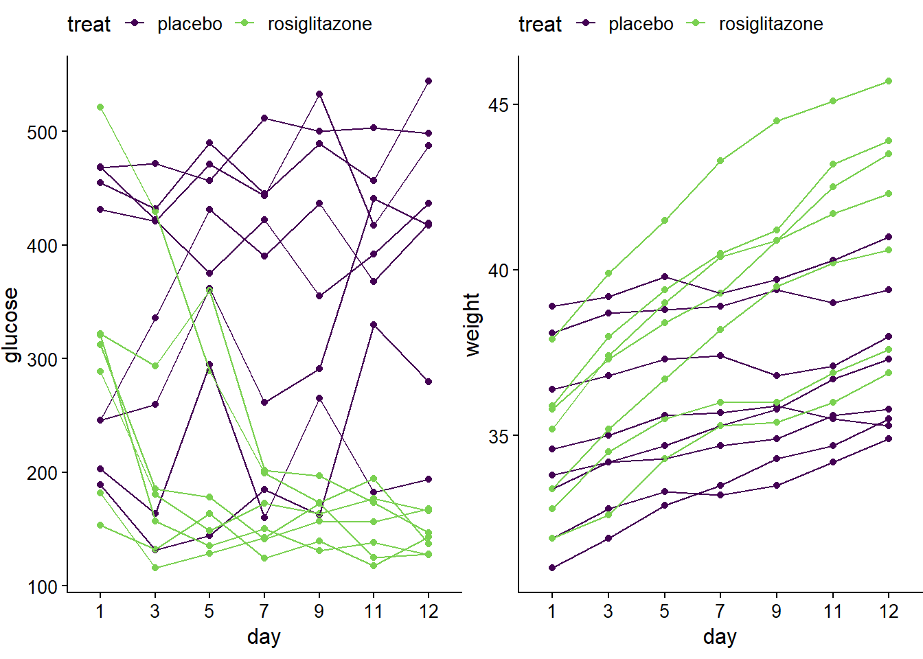
Figure 14.1: Spaghetti plots of jaxwest7 data.
p3 <- ggplot(jw7)+
  geom_histogram(aes(glucose, fill=treat))+
  theme_half_open(12) +
    theme(plot.margin = margin(6, 0, 6, 0), legend.position="top")+
  scale_fill_viridis_d(begin=0, end=0.8)
p4 <- ggplot(jw7)+
  geom_histogram(aes(weight, fill=treat))+
  theme_half_open(12) +
    theme(plot.margin = margin(6, 0, 6, 0), legend.position="top")+
  scale_fill_viridis_d(begin=0, end=0.8)
plot_grid(p3,p4)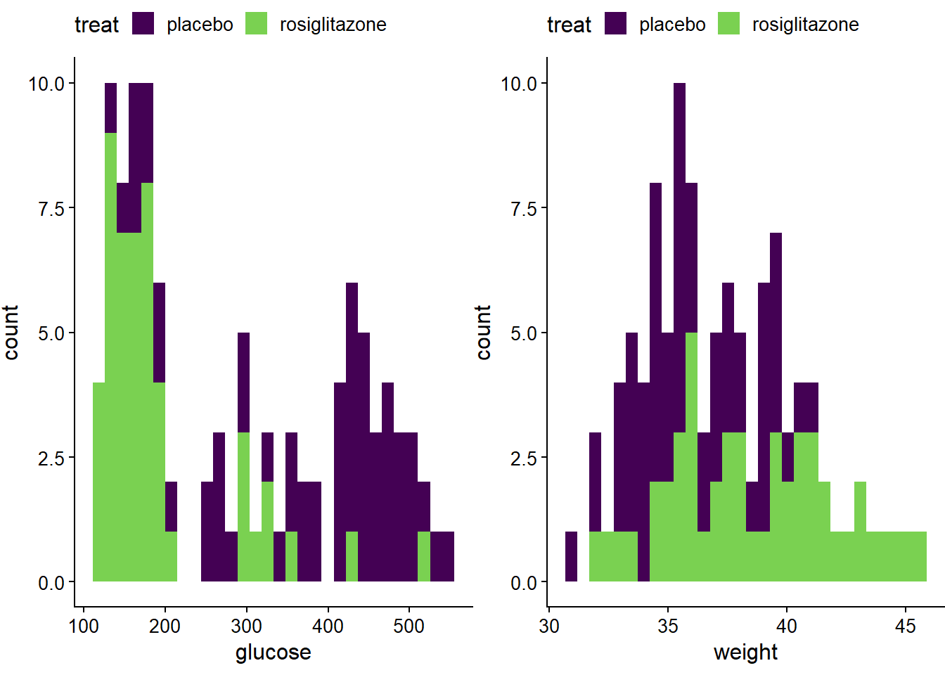
Figure 14.2: Histograms of the jaxwest7 data.
p5 <- ggplot(jw7, aes(day, glucose,color=treat)) +
  stat_summary(fun.data = "mean_sdl",
               fun.args = list(mult = 1),
               geom ="pointrange") +
  stat_summary(fun.y = mean,
               geom = "line",
               aes(group=treat)
               ) +
    theme_half_open(12) +
    theme(plot.margin = margin(6, 0, 6, 0), legend.position="top")+
  scale_color_viridis_d(begin=0, end=0.8)
## Warning: `fun.y` is deprecated. Use `fun` instead.p6 <- ggplot(jw7, aes(day, weight, color=treat)) +
stat_summary(fun.data = "mean_sdl",
fun.args = list(mult = 1),
geom ="pointrange") +
stat_summary(fun.y = mean,
geom = "line",
aes(group=treat)
) +
theme_half_open(12) +
theme(plot.margin = margin(6, 0, 6, 0), legend.position="top")+
scale_color_viridis_d(begin=0, end=0.8)## Warning: `fun.y` is deprecated. Use `fun` instead.plot_grid(p5,p6)## Warning: Computation failed in `stat_summary()`:
## Can't convert a double vector to function## Warning: Computation failed in `stat_summary()`:
## Can't convert a double vector to function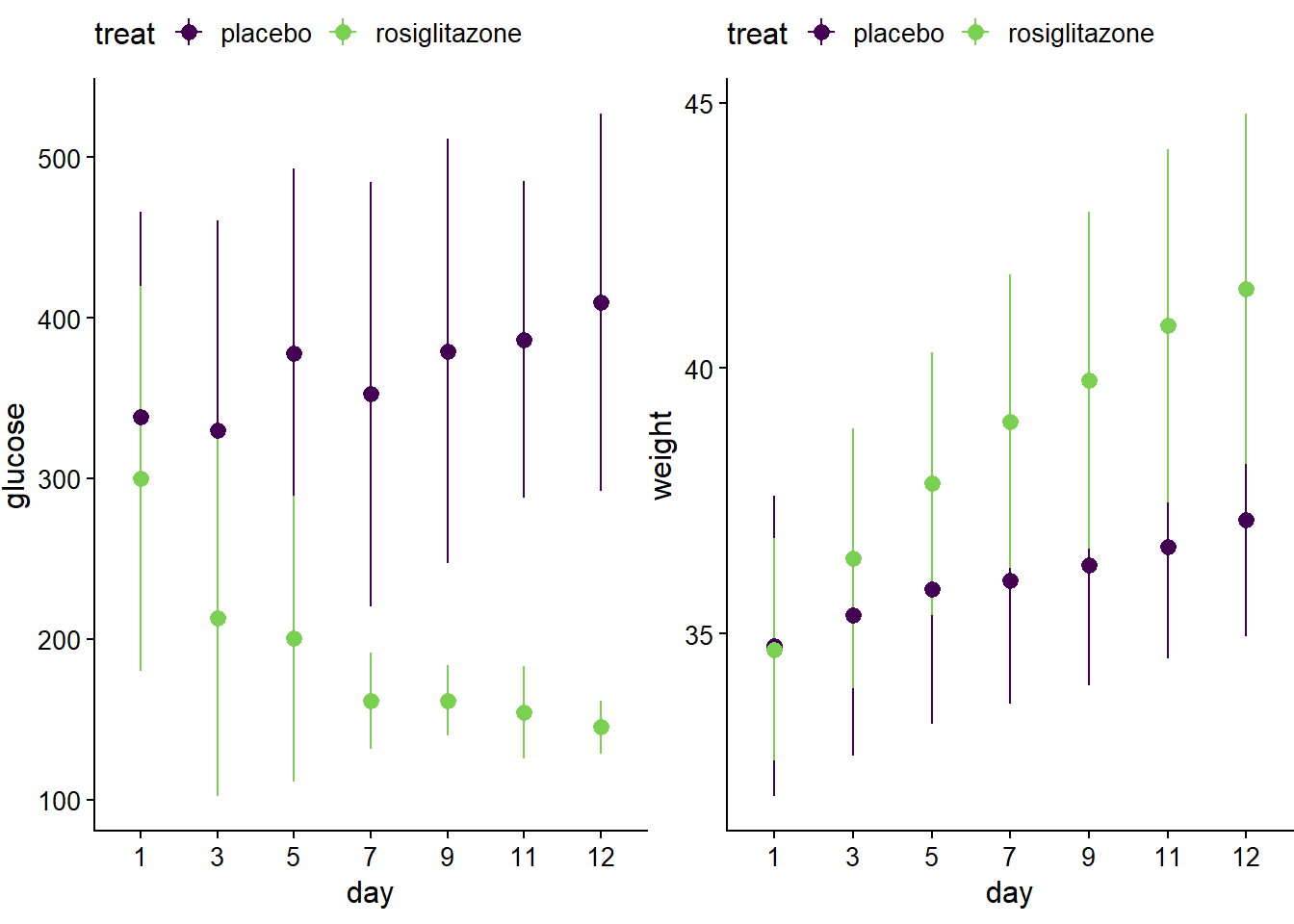
Figure 14.3: Group means and std devs of the jaxwest7 glucose and body weight data.
14.5 Summary
It is important to have a final product in mind before starting a munge. In this case, the goal was to create a dataframe for multivariate statistical analysis. These analyses need for each dependent variable to share a common set of independent variables. That product is the jw7 object above.
* Many data sets are like the Jaxwest7, with plenty of good information but unstructured.
* datapasta is your friend.
* Every munge is a custom munge.