Chapter 36 Reproducible Data Munging Mostly with Tidyverse
library(tidyverse)
library(readxl)
library(viridis)
Reproducibility is when someone who has your data can conduct the same analysis, arriving at the same parameter estimates and conclusions. The data processing steps of an analysis are perhaps the most critical determinant of reproducibility. Ideally, this is performed using a breadcrumbs process, where each step is traceable.
That’s what R scripts do and why they are better than munging data in GUI software, such as excel or other stats packages.
Here’s an example of what I mean by an R script munge. I thought it would be interesting to try and pull this off using mostly tidyverse functions, if possible.
The Jaxwest2 data represent an experiment to establish tumor xenograft growth in \(NOD.CB17-Prkdc^{scid}/J\), an immunodeficient mouse strain.
Jaxwest2 is a nice data set to illustrate a one-way related measures ANOVA. They also provides an opportunity to illustrate some data wrangling technique.
The latter is the focus here. In particular, I’ll illustrate how a complete reproducible data munge can be accomplished using mostly just the tidyverse.
The study design involved injecting HT29 human colon cancer cells into the mice. Over the next few weeks repeated daily measurements were collected from each mouse on a handful of outcome variables, including body weight and tumor lengths, widths, and heights. Tumor volume was calculated from length and width data.
The multiple measures taken from individual subjects are intrinsically-linked. The day of measurement is the only factor, and it has multiple levels. This all fits a one-way repeated measures ANOVA experimental design model.
In the study per se, three groups are compared: 1) Control (no vehicle), 2) Control (vehicle), and 3) Test Group (pretreatment).
The latter is apparently proprietary, providing very little outcome data. The first two are similar and can be expected to generate the same outcomes.
I’m not interested in comparing these groups since the comparisons aren’t particularly interesting scientifically. So we’ll take only the first of these groups to conduct an ANOVA analysis (later). We’ll pretend the other two treatments don’t exist. (Had we compared these groups, too, it would be a two-way ANOVA repeated measures design.)
Therefore, we can use this to study the effect of time on tumor cell growth. We can answer the following scientific question: Will tumor cells grow if injected into the animals?
We’ll focus only on a subset of the data, the tumor volume measurements over time in the first group. This chapter illustrates how to wrangle that subset out from the rest of the data in the excel file.
36.1 Look at the original data carefully
The data are in a file called Jaxwest2.xls, which is available for you on Canvas but can also be downloaded from the Jackson Labs here.
Before starting the munge take a close look at the excel file. It is NOT a cvs file. A few things to note. First, there are two worksheets. One has the experimental data. The second is a variable key.
Now look at that first worksheet. There are two header rows, which is problematic.
The first header row is incomplete since it has no values over the first 7 columns. The label in the 8th column actually refers to header values in the remainder of the columns, not the data beneath it. Those values correspond to the day data were collected in a time series.
The second header row nicely defines the variables for each column. Note how beginning with the 9th column, the variable name incorporates the day number. Thus, bw_1 is the variable body weight on the first day post injection. Thus, the information about the time series is embedded within each variable name.
In other words, most of the variable names are hybrids of two variables, carrying information about both the measurement and the day. That’s actually helpful, but we’ll need to deconvolute those names.
The good news is that the first header row doesn’t provide any information we can’t get from the second header row, so when we read in the data we’ll simply omit that first header row. It would only complicate the munge.
Finally, below the header, every row is a case that corresponds to a unique mouse. The values for the variable mouse_ID illustrates as much.
Here’s the big picture. The column and row structure indicate that repeated measures of multiple outcome variables were collected for each of these mice on each of several days.
36.2 Our goal
Stop me if I’ve used this metaphor previously. But starting a munge is a lot like starting an organic chemistry synthesis. You have the reagents (the excel file, your laptop, and your growing knowledge of R). You know the final product (it needs to be a long table format, with one variable per column).
The only question is how will you create the latter given the former.
In this chapter, let’s collect the time series only for the tumor_vol variable. We’ll ignore all the other outcome variables.
The output–the final goal for now–is to create a plot of the data. Eventually, we’ll run a one-way related measures ANOVA analysis to test whether time has an effect on tumor growth (it does, by the bloody obvious test).
To get there we’ll read in all but the top row of the first sheet of the excel file, then simplify by selecting only the variables that we want from the Jaxwest2 data.
We want a long format data frame where every column represents a unique variable. It will have 1) a numeric tumor volume variable, and 2) a day of measurement variable as a factor, and 3) a variable for the mouse ID also as a factor, and will have data corresponding to only one treatment group (Control (no vehicle)).
36.3 Step 1: Read the data into R
We’ll read in all but the first header row. The function read_excel is from the readxl package, which is part of the tidyverse but you may need to install the package separately. Do so now.
The script below creates the object jw2, which is a data frame of 103 variables.
Look very carefully at those arguments in the read_excel function.
They explain how, except for the first header row, jw2 contains all of the data in the first sheet of the source file.
Skipping a useless, incomplete row helps us immensely. And R is stupid, we have tell it explicitly what sheet to read.
Note that jaxwest2.xls is otherwise untouched. No changes have been made locally to the original source file. That’s important because it is good reproducible practice.
jw2 <-"datasets/jaxwest2.xls" %>%
  read_excel(
    skip=1,
    sheet=1
    )

# remove whitespace
names(jw2) <- str_remove_all(names(jw2)," ")
Note: Here is an optional method to read in the data. In two parts. This forces the bulk of the numeric data to be read in as numeric. You’ll see in a moment why this matters.
right <- read_excel("datasets/jaxwest2.xls", skip=1, sheet=1, range="I2:CY37", col_types="numeric")

left <- read_excel("datasets/jaxwest2.xls", skip=1, sheet=1, range="A2:H37")

alt <- bind_cols(left, right)

names(alt) <- str_remove_all(names(alt), " ")
36.4 Step 2: Select the variables
We slim the jw2 data set considerably using the select function. We don’t have to call it a new object, but that’s done just to illustrate how much better things are compared to the excel file after two simple steps.
We want only the mouse_ID, the test group, and all the columns that correspond to a tumor volume measurement on a given day. We get the latter using the contains function.
We want the mouse_ID because the data are repeated measures. We’ll need it as a grouping variable for both ggplot and ezANOVA.
The test group variable will initially serve as a check to know we grabbed the right data. We can omit it later.
The function contains is super helpful because the tumor volume variables for each day of measurement have a slightly different name, yet each contain the characters tumor_vol_ as a common stem.
Give it a shot. Try to grab a different set of variables using contains.
We’ll create a new object, jw2vol to represent the data only for tumor volumes. Notice how in subsequent chunks jw2vol is modified as we successively munge the data into shape.
jw2vol <- jw2 %>%
  select(
    mouse_ID,
    test_group,
    contains("tumor_vol_")
    )
36.5 Step 3: Trim the cases
As described in the preamble, we only want a subset of the test_groups. We can omit a lot of rows.
Looking at jw2vol we can see those happen to be the first 11 cases in the data set. We’ll slice them out, throwing away the rest.
jw2vol <- jw2vol %>%
  filter(
    test_group == "Control (no vehicle)"
    )
36.6 Step 4: We have a variable problem to fix
Now we have a very simple dataframe with 11 rows and 15 columns. Woot!
But look carefully at the column headers. There is a big problem.
Most of the tumor_vol_ columns are listed as class character variables. They should all be class numeric. Because the tumor_vol variable should be numeric. The only correctly classed numeric variable of them is tumor_vol_19.
What happened??
In a word, *&%!ing NA values.
NA’s caused character coercion: This problem is avoidable by forcing a column type to be numeric on read (see alt above).
We didn’t do that with jw2. If a column of numeric values contains just one non-numeric character, the read_excel function will classify that column as character variable.
We’ve trimmed away a lot of rows and columns since the read step, but the original jaxwest file is full of NAs.
NA values present two problems to solve: a data munging problem and a scientific problem.
And the principles of reproducible data handling demand that we fix both of these problems in R, not in the original data excel data file.
Fix the Munge
We need to convert every tumor_vol column from class_character to class numeric. We’ll get an NA warning but that is OK, we expect it.
jw2vol <- jw2vol %>% mutate_at(vars(tumor_vol_17:tumor_vol_44), as.numeric)## Warning in mask$eval_all_mutate(quo): NAs introduced by coercionjw2vol## # A tibble: 11 x 15
## mouse_ID test_group tumor_vol_17 tumor_vol_18 tumor_vol_19 tumor_vol_22
## <dbl> <chr> <dbl> <dbl> <dbl> <dbl>
## 1 38 Control (no veh~ 27.2 54.8 77.6 104.
## 2 39 Control (no veh~ 12.6 15.8 24.8 36.5
## 3 43 Control (no veh~ NA 30.0 54.9 75.6
## 4 48 Control (no veh~ 7.88 30.2 31.0 53.6
## 5 51 Control (no veh~ 16.2 25.8 28.6 60.6
## 6 58 Control (no veh~ 61.5 105. 93.2 136.
## 7 62 Control (no veh~ 20.1 44.1 60.1 70.3
## 8 63 Control (no veh~ 56.1 93.1 104. 164.
## 9 64 Control (no veh~ 17.1 78.1 79.8 120.
## 10 66 Control (no veh~ 15.1 32.3 35.4 40.3
## 11 67 Control (no veh~ 21.7 27.0 44.6 68.8
## # ... with 9 more variables: tumor_vol_24 <dbl>, tumor_vol_26 <dbl>,
## # tumor_vol_29 <dbl>, tumor_vol_31 <dbl>, tumor_vol_33 <dbl>,
## # tumor_vol_36 <dbl>, tumor_vol_38 <dbl>, tumor_vol_40 <dbl>,
## # tumor_vol_44 <dbl>36.7 Step 5: Impute or Delete
Now that we have numeric variables, we can hunt for NA values within and then do something about it.
First, where are they?
# We couldn't do is.na on character vectors.
# well, we can but it doesn't work, it would yield false negatives

map_df(jw2vol, function(x) sum(is.na(x)))
## # A tibble: 1 x 15
## mouse_ID test_group tumor_vol_17 tumor_vol_18 tumor_vol_19 tumor_vol_22
## <int> <int> <int> <int> <int> <int>
## 1 0 0 1 0 0 0
## # ... with 9 more variables: tumor_vol_24 <int>, tumor_vol_26 <int>,
## # tumor_vol_29 <int>, tumor_vol_31 <int>, tumor_vol_33 <int>,
## # tumor_vol_36 <int>, tumor_vol_38 <int>, tumor_vol_40 <int>,
## # tumor_vol_44 <int>Great! We have only 1 NA. A missing measurement for mouse_ID 43 on day 17.
Impute v Delete
Think of this as a scientific judgment informed by statistical knowledge. Or vice versa.
Leaving the NA value as is will fail the repeated measures statistical analysis. It can’t stand.
The only deletion option involves deleting not just the NA (which is already deleted, but whatev) along with all other values for mouse_ID 43. That throws away 12 other pieces of information just because 1/13 of the information is missing.
Seems extreme.
The other option is to impute. Which is to replace the NA value with a number. Imputing one value in this decent sized data set is not going to cause much bias.
But what number do we use?
One option is to replace the NA with the mean of all other tumor_vols for mouse_ID 43. The other option is to replace using the mean of all other tumor_vols on day 17. In this case, since all later volume measures inflate, the mean of the ID will be biased high.
So we’ll use the mean of the grouped variable instead.
jw2vol <- jw2vol %>% replace_na(
  list(tumor_vol_17 = mean(jw2vol$tumor_vol_17, na.rm=T)))
36.8 Step 6: Go long
The iteration above is 15 columns wide. Next we use the pivot_longer function to make it long. Go here and carefully look at the examples. What happens in this step is just a copy of what they do for their billboard example.
We want a column each for mouse ID, the test group, the day of measurement, and the tumor vol measurement values. The first two of these are done.
The pivot_longer function lets us make the latter two.
jw2vol <- jw2vol %>%

  pivot_longer(cols=starts_with("tumor_vol_"),
    names_to="day",
    names_prefix = "tumor_vol_",
    values_to = "vol",
    values_drop_na = TRUE
  )
jw2vol
## # A tibble: 143 x 4
## mouse_ID test_group day vol
## <dbl> <chr> <chr> <dbl>
## 1 38 Control (no vehicle) 17 27.2
## 2 38 Control (no vehicle) 18 54.8
## 3 38 Control (no vehicle) 19 77.6
## 4 38 Control (no vehicle) 22 104.
## 5 38 Control (no vehicle) 24 89.8
## 6 38 Control (no vehicle) 26 213.
## 7 38 Control (no vehicle) 29 306.
## 8 38 Control (no vehicle) 31 432.
## 9 38 Control (no vehicle) 33 743.
## 10 38 Control (no vehicle) 36 721.
## # ... with 133 more rows36.9 Step 7: Convert other variables to factor
ANOVA are called factorial analyses.
The predictor variable must be a factor. Here, the predictor is day
jw2vol <- jw2vol %>%
  mutate(
    mouse_ID=as.factor(mouse_ID),
    test_group=as.factor(test_group)
    )
jw2vol
## # A tibble: 143 x 4
## mouse_ID test_group day vol
## <fct> <fct> <chr> <dbl>
## 1 38 Control (no vehicle) 17 27.2
## 2 38 Control (no vehicle) 18 54.8
## 3 38 Control (no vehicle) 19 77.6
## 4 38 Control (no vehicle) 22 104.
## 5 38 Control (no vehicle) 24 89.8
## 6 38 Control (no vehicle) 26 213.
## 7 38 Control (no vehicle) 29 306.
## 8 38 Control (no vehicle) 31 432.
## 9 38 Control (no vehicle) 33 743.
## 10 38 Control (no vehicle) 36 721.
## # ... with 133 more rows36.10 Step 8: Plot
Repeated measures on subjects is the primary feature of this data set. Within each mouse_ID, every measurement is intrinsically-related to every other measurement. Point-to-point graphing illustrates this.
This calls for a spaghetti plot.
Here’s all the data! It’s beautiful.
ggplot(jw2vol, aes(as.numeric(day), vol, color=mouse_ID, group=mouse_ID))+
  scale_color_viridis(discrete=T)+
  geom_point(size=2)+
  geom_line()+
  xlab("Day after implant")+
  ylab("Tumor volume")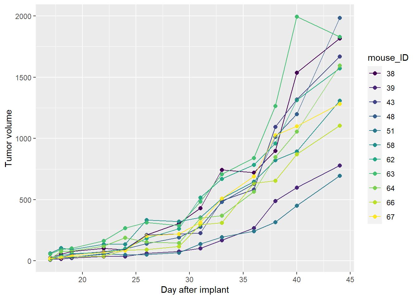
36.11 Step 9: Run the ANOVA
See Chapter 31.