Chapter 15 The Binomial Distribution
library(ggplot2)The binomial probability distribution models the discrete outcomes of dichotomous processes. In other words, events that can be categorized as either a successes or as a failure.
15.1 dbinom
The binomial probability mass function in R is dbinom.
R’s dbinom function returns p(x), a probability value produced by the binomial probability mass function: \[p(x)={n\choose x}(p)^x(1-p)^{(n-x)}\]
Where \(n\) is the number of trials, \(x\) is the value of the number of successes, \(p\) is the probability of a single success, and therefore \(1-p\) is the probability of a single failure.
The coin toss serves as the classic explainer for binomial events. A fair coin can land as either heads, or tails with equal probabilities. Unless you’re Patriot’s quarterback Tom Brady, for whom it always lands as heads.
If Matt Ryan tossed a coin 10 times, what’s the probability of him getting EXACTLY 7 heads?
dbinom(x=7, size=10, prob=0.5)## [1] 0.1171875That’s almost a 12% chance! Eight heads would be even more unlikely. And so on.
Female mice enter estrus one out of five days. This implies that if a female mouse is mated on any random day, the probability of any single mating resulting in pregnancy is 0.2.
On a given day, if you set up 12 female mize for mating, what’s the probability that exactly half of them would become pregnant?
dbinom(x=6, size=12, prob=0.2)## [1] 0.01550215There’s only a 1.55% chance of getting EXACTLY 6 dams out of that mating set up.
The script below illustrates the probabilities over a full range of possible pregnancy outcomes, for a trial of size 12 (ie, 12 matings set up)
x <- 1:10
size <- 12
prob <- 0.2

df <- data.frame(x, px=dbinom(x, size, prob))

ggplot(df, aes(x, px)) +
  geom_col(fill ="blue") +
  xlab("x, number of successes") +
  ylab("p(x)") +
  labs(title = paste("dbinom","(","trial size=",size,",","p=",prob,")"))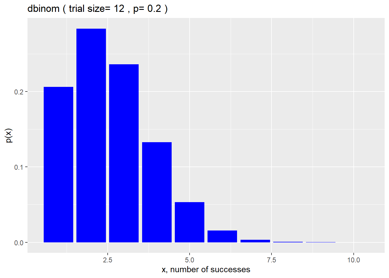
It’s evident that binomial distributions where the probabilities of successes and failures are uneven are skewed. The only way to make these appear more normally distributed is to have equal probabilities for successes and failures.
15.2 pbinom
R’s pbinom is the cumulative probability distribution function for the binomial. \[p(x)={\sum_{i=0}^{x}}{n\choose i}(p)^i(1-p)^{(n-i)}\]
This function returns the cumulative probability value for a number of successes in n trials. This can be a very useful value to model.
For example, if you set up 12 matings of mice, where each had a 0.2 probability of pregnancy, what is the probability that you would have up to 6 pregnant dams?
pbinom(6, 12, 0.2, lower.tail=T)## [1] 0.9960969There’s is a very high probability of getting UP TO 6 pregnancies from 12 matings!
If we turn the lower.tail argument from TRUE to FALSE the pbinom returns a p-value like probability.
What’s the probability of getting 6 or more pregnancies from 12 matings where the probability of a single pregnancy is 0.2?
pbinom(6, 12, 0.2, lower.tail=F)## [1] 0.003903132That’s about 0.39%! Which would be a very rare outcome from the mating trial, indeed! Maybe even scientifically significant were it to occur.
Perhaps it’s useful to visualize both the upper and lower tails of this cumulative function:
q <- 1:10
size <- 12
prob <- 0.2

df <- data.frame(q, px=pbinom(q, size, prob))

ggplot(df, aes(q, px)) +
  geom_col(fill ="blue") +
  xlab("x, number of successes") +
  ylab("p(x)") +
  labs(title = paste("pbinom","(","trial size=",size,",","p=",prob,"lower.tail=TRUE",")"))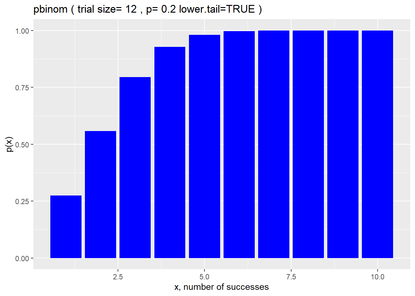
df <- data.frame(q, px=pbinom(q, size, prob, lower.tail=F))

ggplot(df, aes(q, px)) +
  geom_col(fill ="blue") +
  xlab("x, number of successes") +
  ylab("p(x)") +
  labs(title = paste("pbinom","(","trial size=",size,",","p=",prob,"lower.tail=FALSE",")"))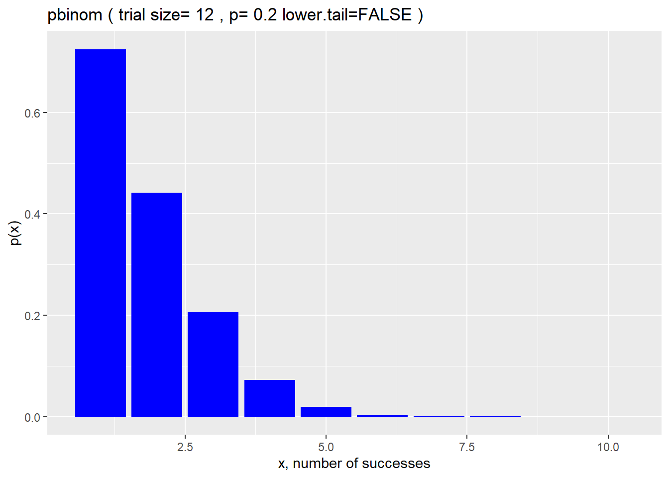
15.3 qbinom
The quantile binomial distribution function in R is qbinom.
qbinom is the inverse of the pbinom function. This predicts the number of successes that might occur given a percentile of the distribution.
Assuming 12 matings are set up, where the probability of any one pregnancy success is 0.2, what number of pregnancies would be expected if the group performed at the 90th percentile?
qbinom(p=0.90, size=12, prob=0.2, lower.tail=T)## [1] 4That’s only 4 litters. That should make sense, since only 1 in 5 would be pregnant on average. To out perform this expectation at the 90th percentile is still not a very large numer
The graph below illustrates this. Notice the step-wise distribution, which is diagnostic of discrete functions.
#define variables
p <- seq(0, .99, 0.03) #cumulative probability quantiles
size <- 12 #number of trials
prob <- 0.2 #probability of success of one trial

df <- data.frame(p, q=qbinom(p, size, prob))

ggplot(df, aes(p, q)) +
  geom_col(fill="blue") +
  xlab("p(q)") +
  ylab("q") +
  labs(title = paste("qbinom","(","trial size=",size,",","p=",prob,")"))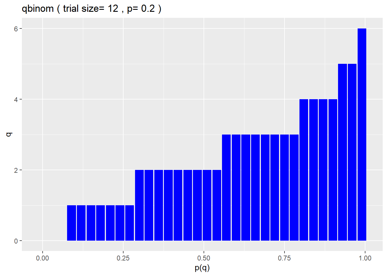
15.4 rbinom
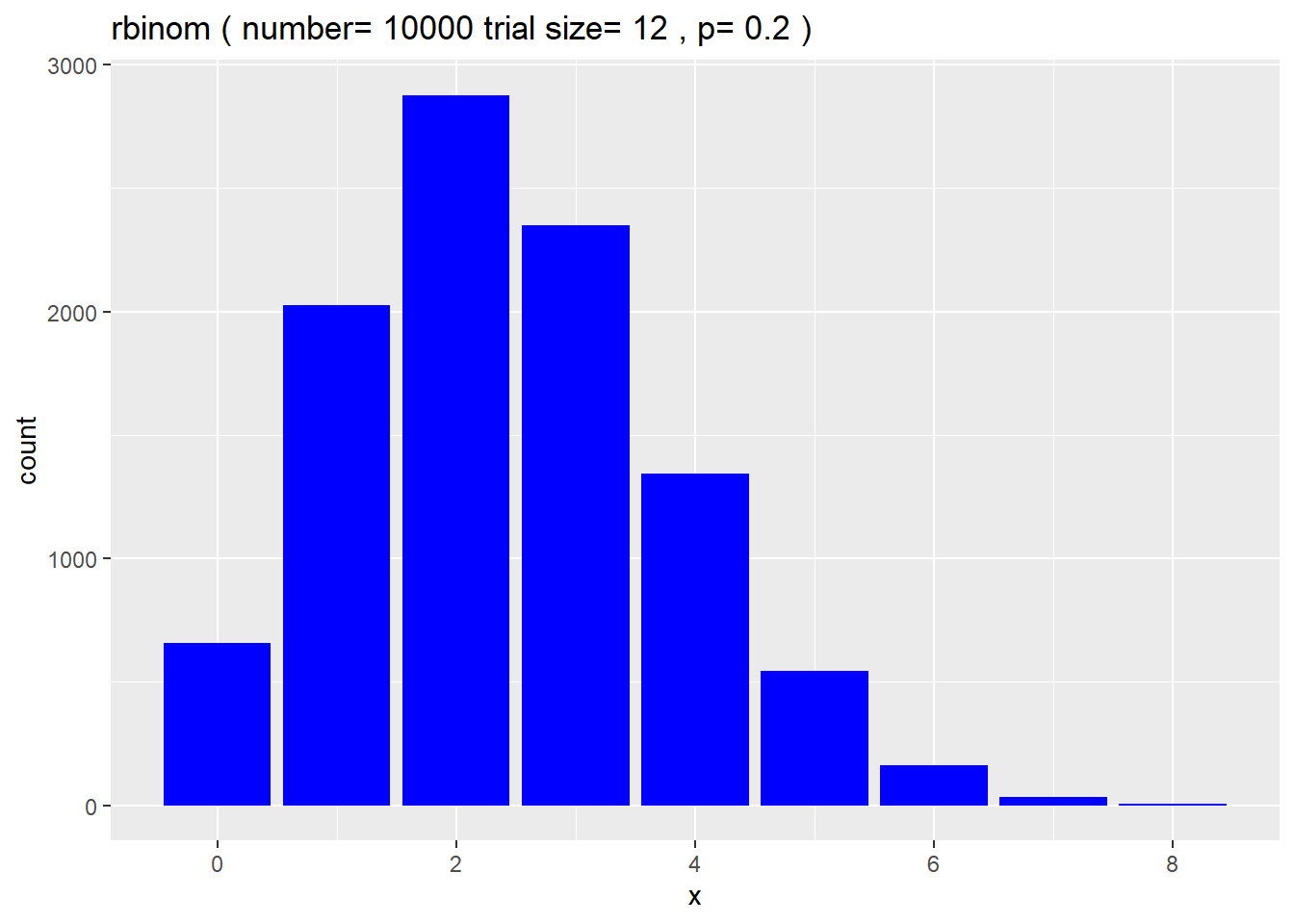
The rbinom function is for random simulation of n binomial trials of a given size and event probability. The output is the number of successful events per trial.
Let’s simulate 12 matings 12 times, as if we do one a mating involving 12 females, once per month. How many successes will we see per month?
The output below represents the number of litters we would produce on each of those months. The point is, we don’t get the average every month. Some times its more successes, others its fewer. Models are perfect, data are not.
rbinom(n=12, size=12, prob=0.2)## [1] 1 4 3 2 3 3 0 5 1 1 3 4Here’s a histogram from a very large number of simulations of the same scenario. You can clearly see the binomial distribution for this trial size and probability of success is skewed. You can also clearly see the average of the distribution…which is somewhere between 2 and 3.
n <- 10000 #number of simulations
size <- 12 #number of trials
prob <- 0.2 #probability of success of one trial

df <- data.frame(x=rbinom(n, size, prob)) #x=number of successful trials

ggplot(data=df, aes(df$x)) +
  stat_count(fill="blue") +
  xlab("x")+
  ylab("count")+
  labs(title = paste("rbinom","(","number=",n,"trial size=",size,",","p=",prob,")"))
## Warning: Use of `df$x` is discouraged. Use `x` instead.