Chapter 22 Signed Rank Distribution
The signed rank per se represents a type of data transformation. Experimental data are first transformed into signed ranks (see below). When signed ranks for a group of data are summed that sum serves as a test statistic. The sign rank test has a symmetrical normal-like distribution, which is discrete rather than continuous.
In R, when using the wilcox.test to evaluate data from one sample or for paired sample nonparametric designs, the sums of only the postive signed ranks are calculated as the test statistic \(V\).
The distribution of \(V\) is the focus of this document.
There is a unique sign rank sum distribution for sample size \(n\). These represent the distributions that would be expected under the null hypothesis.
In practice, values of \(V\) that are on the extreme ends of these distributions can have p-values that are so low that we would reject the null \(V\) distribution as a model for our dataset and accept an alternative.
The use of \(V\) as a test statistic and its null distributions can be a bit confusing if you’ve worked with other software to do nonparametric hypothesis testing.
For example, Prism reports \(W\) as a test statistic for sign rank-based nonparametric experimental designs. On that platform, \(W\) is the sum of all signed ranks, not just the positives. The center location of \(W\) as a sign rank test statistic is at or near zero on the \(W\) distributions, whereas zero is the lowest possible value for \(V\). Although calculated slightly differently, \(W\) and \(V\) are equivalent ways to express the same relationship between the values within the original dataset.
22.1 Transformation of data into sign ranks
22.1.1 For a one group sample
A one group sample represents a single vector of data values.
Let a sample of size \(n\) for a variable \(X\) take on the values \(x_1, x_2, ... x_n\). The location of this vector will be compared to a location value \(x = \mu\), such that \(z_i=x_i-\mu\) for \(i=1\ to\ n\).
To transform the sample to a vector of signed ranks, first rank \(|z_i|\) from lowest to highest. \(R_i\) is the rank value for each value of \(|z_i|\). \(\psi = 0\) if \(z_i < \mu\), or \(\psi= 1\) if \(z_i > \mu\). The signed ranks of the original vector values are therefore \(R_1\psi, R_2\psi,...R_n\psi\).
22.1.2 For a paired sample
The differences between paired groups in an experimental sample also represent a single vector of data values, which explains why a sign rank-based test are used, rather than a rank sum test.
A sample of \(n\) pairs of the variables \(X\) and \(Y\) has the values \((x_1,y_1); (x_2,y_2); ... (x_n,y_n)\). The difference between the values of \(X\) and \(Y\) will be compared to zero. For \(i=1\ to\ n\), the difference is \(z_i=x_i-y_i\).
The sign rank transformation of \(z_i\) for each pair is performed as above.
22.1.3 The sign rank test statistic in R
The sign rank test statistic for both the one- and two-sample cases is \(V = \sum_i^{n}R_i\psi_{>0}\), which has a symmetric distribution ranging from a minimum of \(V = 0\) to a maximum of \(V = \frac{n(n+1)}{2}\).
This test statistic is produced by the wilcox.test for one-sample and paired-sample expriments. Again, \(V\) is the sum of the positive signed-ranks only. Other softer produces a test statistic \(W\), which is the sum of all the signed ranks
22.1.3.1 More about the test statistic
The expectation of \(V\) (ie, its median) when the null hypothesis is true is \(E_0(V)=\frac{n(n+1)}{4}\) and its variance is \(var_0(V)=\frac{n(n+1)(2n+1)}{24}\)
The standardized version of \(V\) is \(V^*=\frac{V-E_0(V)}{var_0(V)}\). As \(n\) gets large, \(V^*\) asymptotically approaches a normal distribution \(N(0,1)\).
Zero and tied values of \(|Z_i|\) occur in datasets for both the one group and paired group transformations of raw data. When values of \(|Z|=0\) occur, they are discarded in the calculation of \(V\) and the \(n\) is readjusted.
The integer value of ranks for tied \(|Z's|\) are averaged. Although these ties don’t change \(E_0(V)\), they do reduce the variance of \(V\). \(var_0(V)=\frac{n(n+1)(2n+1)-\frac{1}{2}\sum_{j=1}^{g}t_j(t_j-1)(t_j+1)}{24}\)
22.2 R’s Four Sign Rank Distribution Functions
22.2.1 dsignrank
The function dsinerank returns a probability value given two arguments: \(x\) is an integer value, meant to represent \(V\), which is the value of the sign rank test statistic; and \(n\) is the sample size of either a one-sample or a paired experiment.
The probabilities for individual values of \(V\) are sometimes useful to calculate. For example, the probability of obtaining \(V=3\) for an \(n\)=10 experiment is:
dsignrank(3, 10)## [1] 0.001953125More ofen it is useful to visualize the null distribution of the sign rank test statistic over a range of values. Here’s a distribution of \(V\) for an experiment of sample size 10.
n <- 10 #number of independent replicates in experiment
max <- n*(n+1)/2
df <- data.frame(pv=dsignrank(c(0:max), n))
ggplot(df, aes(x=c(0:max), pv)) +
  geom_col() + xlab("V") + ylab("p(V)")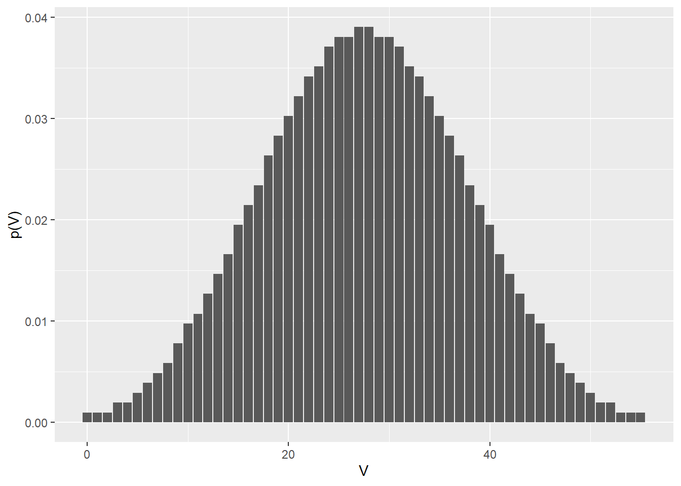
22.2.2 psignrank
This is the cumulative distribution function for the sign rank test statistic. \(q\) is an integer to represent the expected value of \(V\), and \(n\) is the sample size. Given these arguments, psignrank will return a p-value for a given test statistic value. psignrank returns the sum of the probabilities of \(V\) over a range, and is reversible using the lower.tail argument.
Here we use psignrank to generate the p-value when \(V\)=3 and \(n\)=1. Then we show the sum of the dsignrank output for \(V\)=0:3 is equal to psignrank. Finally, the symmetry of the distribution is illustrated:
psignrank(3, 10, lower.tail=T)## [1] 0.004882812sum(dsignrank(c(0:3), 10)) == psignrank(3, 10, lower.tail=T)## [1] TRUEpsignrank(51, 10, lower.tail=F)## [1] 0.004882812psignrank(51, 10, lower.tail=F)==psignrank(3, 10, lower.tail=T)## [1] TRUEThe distributions of psignrankfor its lower and upper tails:
n <- 10
max <- n*(n+1)/2
df <- data.frame(pv=psignrank(c(0:max), n))
ggplot(df, aes(x=c(0:max), pv)) +
  geom_col() + xlab("V") + ylab("p-value for V")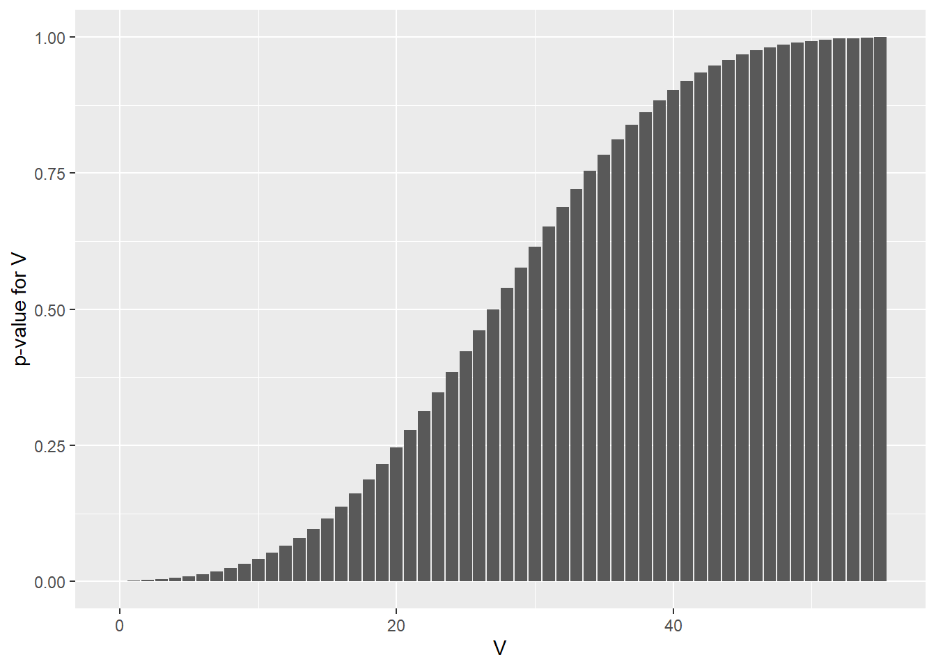
df <- data.frame(pv=psignrank(c(0:max), n, lower.tail=F))
ggplot(df, aes(x=c(0:max), pv)) +
  geom_col() + xlab("V") + ylab("p-value for V")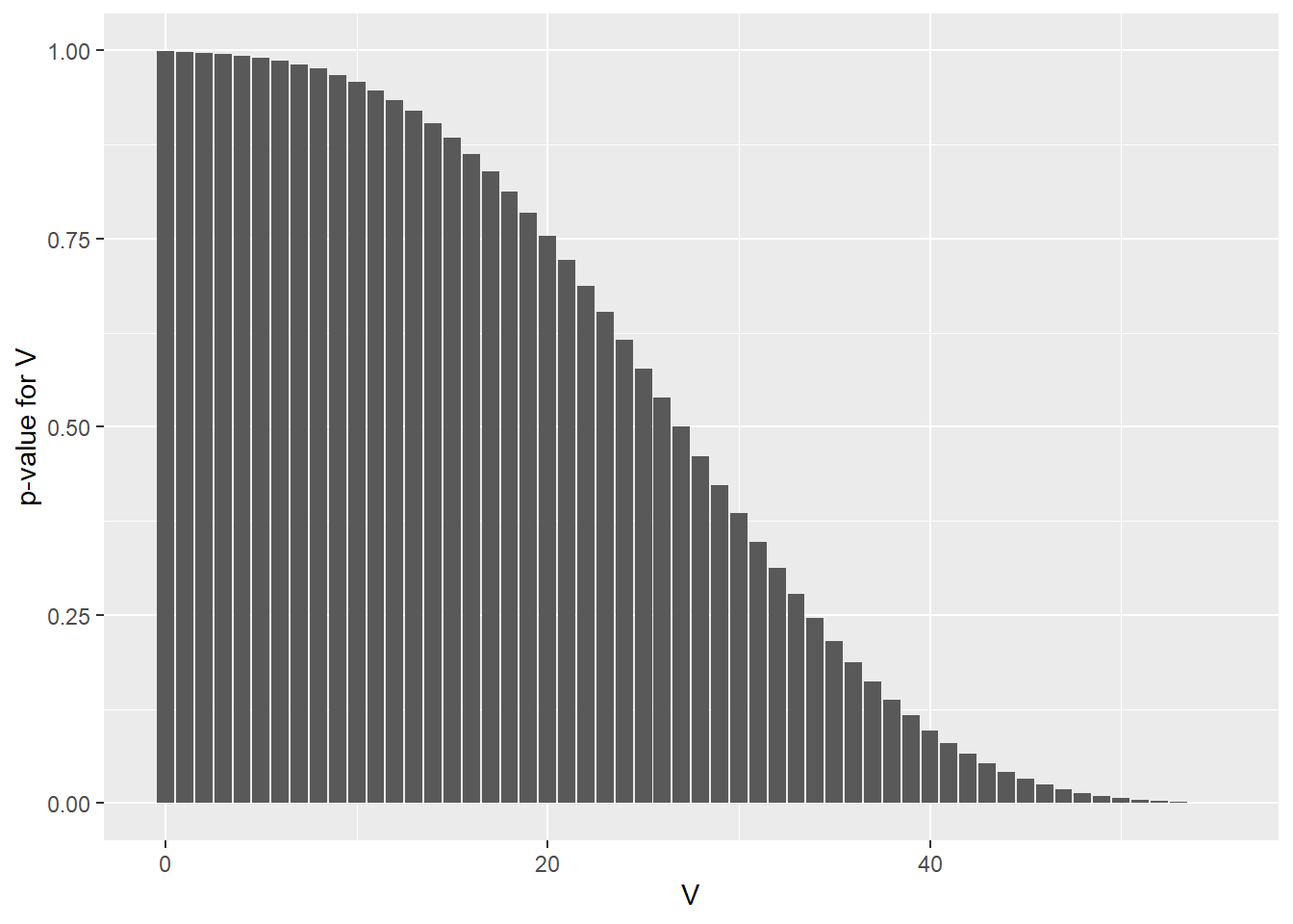
22.2.3 qsignrank
This is the quantile signrank function in R. If given a quantile value (eg, 2.5%) and sample size \(n\), qsignrank will return the value of the test statistic V.
For example, here is how to find the critical limits for a two-sided hypothesis test for an experiment with 10 independent replicates, when the type1 error of 5% is evenly distributed to both sides:
qsignrank(0.025, 10, lower.tail=T)## [1] 9qsignrank(0.025, 10, lower.tail=F)## [1] 46Interpretation of critical limits output: When the null two-sided hypothesis is true, \(9\le V\le46\). In other words, the null hypothesis would not be rejected if an experiment generated a \(V\) between 9 and 46.
Alternative interpretation: \(p<0.05\) when \(9>V>46\). In other words, a two sided null hypothesis would be rejected if it generated a \(V\) below 9 or greater than 46.
And here are the critical limits for one-sided hypothesis tests for an experiment with 10 independent replicates, when the type1 error is 5%. Notice how the critical limits differ between one-sided and two-sided tests:
qsignrank(0.05, 10, lower.tail=T)## [1] 11qsignrank(0.05, 10, lower.tail=F)## [1] 44Standard interpretion: For one-sided type1 error of 5%, When the null hypothesis is true, \(V\ge11\), or \(V\le44\).
Alternative interpretation: \(p < 0.05\) when \(V< 11\) or \(V>44\)
Here is a graphical representation of the qsignrank function. Note the stairstep pattern, characteristic of discrete distributions:
n <- 10
x <- seq(0,1,0.01)
df <- data.frame(v=qsignrank(x, n, lower.tail=T))
ggplot(df, aes(x=x, v)) +
  geom_point() + xlab("p-value") + ylab("V")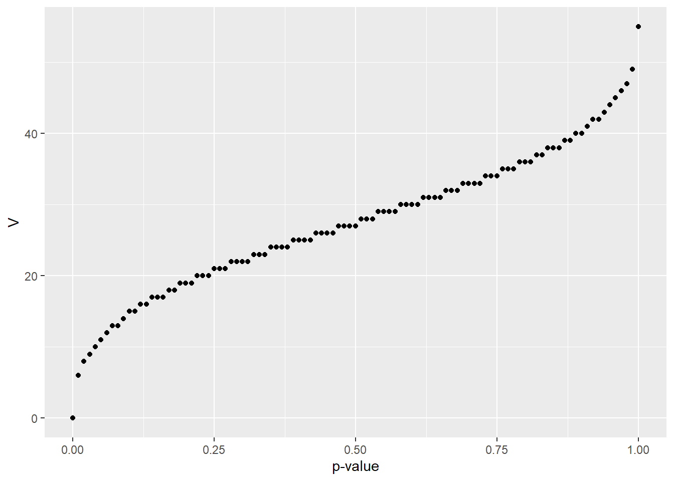
22.2.4 rsignrank
This function is used to simulate random values of the test statistic for null distributions for \(V\).
Here’s a group of 5 random values from a distribution for a sample size of 10. The output values represent the sum of the positive sign ranks, aka the \(V\) test statistic values that would be generated from doing 10 different random experiments of this sample size…if the null hypothesis were true:
rsignrank(5, 10)## [1] 35 30 35 43 24Let’s simulate 1,000,000 such experiments. And then let’s count the number of extreme values of \(V\) that would randomly occur in that number of experiments.
We know from the qsignrank function that 11 is the critical value for a one-sided test at \(\alpha=0.05\) for a sample size of 10.
Thus,our “significance test” for each of the 1,000,000 random experiments is to ask whether \(V\) is below the critical value of 11 for that sample size.
Given we’ve set a 5% false positive rate, we’d expect to see around 50000 false positives (5% of 1,000,000):
sim <- rsignrank(1000000, 10)
test <- sim<11
length(which(test==TRUE))
## [1] 42334If you ran that chunk repeatedly you’d come up with something around 4.2% each time. Why is it not exactly 5%? What do you think that means? Are there experimental sample-sizes where the type1 error would be even further or closer to 5%?