Chapter 50 RNA-seq with R
library(tidyverse)
library(edgeR)
library(limma)
library(gplots)
library(viridis)
This example is adopted extensively from RNA-seq analysis in R by Belinda Phips and colleagues. The data are available here and here.
These are part of a broader workship presented by the group with very easy to follow protocols for RNA-seq analysis with R. There is a publication, also
The data below are from a study of mammary gland development showing the pro-survival gene Mcl1 as a master regulator gland development. They represent duplicate RNA-seq measurements from each of 6 groups: basal and luminal cells from virgin, pregnant and lactating mice.
The purpose of having this in JABSTB at this stage is to offer a gentle introduction to RNA-seq data and analysis. The focus here is on the classification methods within this example. Differential gene expression and pathway analysis is not covered here.
50.1 Overview
Remember organic chemistry? We have reagents. We have a specific product in mind. We do a series of reactions/cleanup steps toward that end product.
Analyzing gene expression data is no different.
The end product to shoot for here is a hierarchical cluster.
The reagents are a file of raw RNAseq counts per gene per replicate. We also have a file with some additional information about each replicate…metadata. We’ll need to merge the metadata of the 2nd file into the first, the gene expression data.
As for the counts, we’ll need to remove genes with missing or low values. Ultimately the counts will be log transformed, so they become Gaussian-distributed data. That’s necessary for the clustering (or other statistical models), which assumes Gaussian distributed input.
50.2 Install Bioconductor
This chapter uses functions in Bioconductor.
Bioconductor is a universe of packages and functions geared for bio/omics data analysis. It is managed separately from the broader CRAN package universe.
Just as for the CRAN universe, we don’t automagically have the full universe of Bioconductor packages by default. We just get a working base suite. If we want more, we have to find it and install it.
The most important difference is to use the Bioconductor package manager to install Bioconductor packages.
When we want to install additional Bioconductor packages we would do so this way, BiocManager::install("newthing"), not this way, install.packages("newthing")
Go to that link above and read more about Bioconductor.
There is much to install. This will take a while.
A warning: Do NOT compile anything
If you see the prompt below, always choose no:
Do you want to install from sources the package which needs compilation (yes/no/cancel)?
Clear?
Then go install Bioconductor by running the script below in your console. Copy/paste the full script into your console. Remove the # symbols. Then press enter.
# if (!requireNamespace("BiocManager", quietly = TRUE))
#     install.packages("BiocManager")
# BiocManager::install(version = "3.13")
50.3 Import raw count data
By this point, there has already been considerable bioinformatical processing of the raw sequence data. Sequences have been matched to their genes and to each other. Those methods are beyond the scope of what we want to cover here.
Chances are the RNAseq core facility will have done the bioinformatics for the customer. Typically, they provide the researcher a file of counts, such as this one, as a minimal deliverable.
The values in this table are counts of the number of transcript reads per gene, in each of the 12 samples. They are in a delimited file format, so we use the read.delim function.
Read them into an object.
seqdata <- read.delim("datasets/GSE60450_Lactation-GenewiseCounts.txt")
head(seqdata)
## EntrezGeneID Length MCL1.DG_BC2CTUACXX_ACTTGA_L002_R1
## 1 497097 3634 438
## 2 100503874 3259 1
## 3 100038431 1634 0
## 4 19888 9747 1
## 5 20671 3130 106
## 6 27395 4203 309
## MCL1.DH_BC2CTUACXX_CAGATC_L002_R1 MCL1.DI_BC2CTUACXX_ACAGTG_L002_R1
## 1 300 65
## 2 0 1
## 3 0 0
## 4 1 0
## 5 182 82
## 6 234 337
## MCL1.DJ_BC2CTUACXX_CGATGT_L002_R1 MCL1.DK_BC2CTUACXX_TTAGGC_L002_R1
## 1 237 354
## 2 1 0
## 3 0 0
## 4 0 0
## 5 105 43
## 6 300 290
## MCL1.DL_BC2CTUACXX_ATCACG_L002_R1 MCL1.LA_BC2CTUACXX_GATCAG_L001_R1
## 1 287 0
## 2 4 0
## 3 0 0
## 4 0 10
## 5 82 16
## 6 270 560
## MCL1.LB_BC2CTUACXX_TGACCA_L001_R1 MCL1.LC_BC2CTUACXX_GCCAAT_L001_R1
## 1 0 0
## 2 0 0
## 3 0 0
## 4 3 10
## 5 25 18
## 6 464 489
## MCL1.LD_BC2CTUACXX_GGCTAC_L001_R1 MCL1.LE_BC2CTUACXX_TAGCTT_L001_R1
## 1 0 0
## 2 0 0
## 3 0 0
## 4 2 0
## 5 8 3
## 6 328 307
## MCL1.LF_BC2CTUACXX_CTTGTA_L001_R1
## 1 0
## 2 0
## 3 0
## 4 0
## 5 10
## 6 342As usual, let’s take some time to inspect the data.
To see the data set’s dimensions.
dim(seqdata)## [1] 27179 14There are 14 columns and over 27000 rows.
To see the data set’s class.
class(seqdata)## [1] "data.frame"To see the column/row structure of this object.
head(seqdata)## EntrezGeneID Length MCL1.DG_BC2CTUACXX_ACTTGA_L002_R1
## 1 497097 3634 438
## 2 100503874 3259 1
## 3 100038431 1634 0
## 4 19888 9747 1
## 5 20671 3130 106
## 6 27395 4203 309
## MCL1.DH_BC2CTUACXX_CAGATC_L002_R1 MCL1.DI_BC2CTUACXX_ACAGTG_L002_R1
## 1 300 65
## 2 0 1
## 3 0 0
## 4 1 0
## 5 182 82
## 6 234 337
## MCL1.DJ_BC2CTUACXX_CGATGT_L002_R1 MCL1.DK_BC2CTUACXX_TTAGGC_L002_R1
## 1 237 354
## 2 1 0
## 3 0 0
## 4 0 0
## 5 105 43
## 6 300 290
## MCL1.DL_BC2CTUACXX_ATCACG_L002_R1 MCL1.LA_BC2CTUACXX_GATCAG_L001_R1
## 1 287 0
## 2 4 0
## 3 0 0
## 4 0 10
## 5 82 16
## 6 270 560
## MCL1.LB_BC2CTUACXX_TGACCA_L001_R1 MCL1.LC_BC2CTUACXX_GCCAAT_L001_R1
## 1 0 0
## 2 0 0
## 3 0 0
## 4 3 10
## 5 25 18
## 6 464 489
## MCL1.LD_BC2CTUACXX_GGCTAC_L001_R1 MCL1.LE_BC2CTUACXX_TAGCTT_L001_R1
## 1 0 0
## 2 0 0
## 3 0 0
## 4 2 0
## 5 8 3
## 6 328 307
## MCL1.LF_BC2CTUACXX_CTTGTA_L001_R1
## 1 0
## 2 0
## 3 0
## 4 0
## 5 10
## 6 342We can see that 2 columns are not like the others. We’ll deal with that below to create a data object that has row names and column names and where all the numeric values in the columns are sequence counts.
A second delimited text file has additional factorial information about each sample replicate. Including some important independent variables that are factorial. It will be used later as a key aspect of interpreting the cluster analysis. But read it into the environment now and have a look.
sampleinfo <- read.delim("datasets/SampleInfo_Corrected.txt")
sampleinfo
## FileName SampleName CellType Status
## 1 MCL1.DG_BC2CTUACXX_ACTTGA_L002_R1 MCL1.DG basal virgin
## 2 MCL1.DH_BC2CTUACXX_CAGATC_L002_R1 MCL1.DH basal virgin
## 3 MCL1.DI_BC2CTUACXX_ACAGTG_L002_R1 MCL1.DI basal pregnant
## 4 MCL1.DJ_BC2CTUACXX_CGATGT_L002_R1 MCL1.DJ basal pregnant
## 5 MCL1.DK_BC2CTUACXX_TTAGGC_L002_R1 MCL1.DK basal lactate
## 6 MCL1.DL_BC2CTUACXX_ATCACG_L002_R1 MCL1.DL basal lactate
## 7 MCL1.LA_BC2CTUACXX_GATCAG_L001_R1 MCL1.LA luminal virgin
## 8 MCL1.LB_BC2CTUACXX_TGACCA_L001_R1 MCL1.LB luminal virgin
## 9 MCL1.LC_BC2CTUACXX_GCCAAT_L001_R1 MCL1.LC luminal pregnant
## 10 MCL1.LD_BC2CTUACXX_GGCTAC_L001_R1 MCL1.LD luminal pregnant
## 11 MCL1.LE_BC2CTUACXX_TAGCTT_L001_R1 MCL1.LE luminal lactate
## 12 MCL1.LF_BC2CTUACXX_CTTGTA_L001_R1 MCL1.LF luminal lactate50.4 Munge to simpler table
Create a table that has only count data so that we can do several manipulations of the gene expression data.
countdata <- seqdata[, 3:14]Have a look so we can confirm we no longer have the first two columns.
head(countdata)## MCL1.DG_BC2CTUACXX_ACTTGA_L002_R1 MCL1.DH_BC2CTUACXX_CAGATC_L002_R1
## 1 438 300
## 2 1 0
## 3 0 0
## 4 1 1
## 5 106 182
## 6 309 234
## MCL1.DI_BC2CTUACXX_ACAGTG_L002_R1 MCL1.DJ_BC2CTUACXX_CGATGT_L002_R1
## 1 65 237
## 2 1 1
## 3 0 0
## 4 0 0
## 5 82 105
## 6 337 300
## MCL1.DK_BC2CTUACXX_TTAGGC_L002_R1 MCL1.DL_BC2CTUACXX_ATCACG_L002_R1
## 1 354 287
## 2 0 4
## 3 0 0
## 4 0 0
## 5 43 82
## 6 290 270
## MCL1.LA_BC2CTUACXX_GATCAG_L001_R1 MCL1.LB_BC2CTUACXX_TGACCA_L001_R1
## 1 0 0
## 2 0 0
## 3 0 0
## 4 10 3
## 5 16 25
## 6 560 464
## MCL1.LC_BC2CTUACXX_GCCAAT_L001_R1 MCL1.LD_BC2CTUACXX_GGCTAC_L001_R1
## 1 0 0
## 2 0 0
## 3 0 0
## 4 10 2
## 5 18 8
## 6 489 328
## MCL1.LE_BC2CTUACXX_TAGCTT_L001_R1 MCL1.LF_BC2CTUACXX_CTTGTA_L001_R1
## 1 0 0
## 2 0 0
## 3 0 0
## 4 0 0
## 5 3 10
## 6 307 342Now let’s place the EntrezGeneID values back in, but as row names. The row names are not a variable.
rownames(countdata) <- seqdata[,1]Check it out.
head(countdata)## MCL1.DG_BC2CTUACXX_ACTTGA_L002_R1 MCL1.DH_BC2CTUACXX_CAGATC_L002_R1
## 497097 438 300
## 100503874 1 0
## 100038431 0 0
## 19888 1 1
## 20671 106 182
## 27395 309 234
## MCL1.DI_BC2CTUACXX_ACAGTG_L002_R1 MCL1.DJ_BC2CTUACXX_CGATGT_L002_R1
## 497097 65 237
## 100503874 1 1
## 100038431 0 0
## 19888 0 0
## 20671 82 105
## 27395 337 300
## MCL1.DK_BC2CTUACXX_TTAGGC_L002_R1 MCL1.DL_BC2CTUACXX_ATCACG_L002_R1
## 497097 354 287
## 100503874 0 4
## 100038431 0 0
## 19888 0 0
## 20671 43 82
## 27395 290 270
## MCL1.LA_BC2CTUACXX_GATCAG_L001_R1 MCL1.LB_BC2CTUACXX_TGACCA_L001_R1
## 497097 0 0
## 100503874 0 0
## 100038431 0 0
## 19888 10 3
## 20671 16 25
## 27395 560 464
## MCL1.LC_BC2CTUACXX_GCCAAT_L001_R1 MCL1.LD_BC2CTUACXX_GGCTAC_L001_R1
## 497097 0 0
## 100503874 0 0
## 100038431 0 0
## 19888 10 2
## 20671 18 8
## 27395 489 328
## MCL1.LE_BC2CTUACXX_TAGCTT_L001_R1 MCL1.LF_BC2CTUACXX_CTTGTA_L001_R1
## 497097 0 0
## 100503874 0 0
## 100038431 0 0
## 19888 0 0
## 20671 3 10
## 27395 307 342The object countdata is a data frame. Now with row and column names. Each column corresponds to a biological replicate, each row a gene id. Every cell in a row is the raw transcript counts for that gene for that replicate condition.
One last touch. The long column names are annoying. Let’s shorten the column names. They start with 7 non-identical characters which are good identifiers for each replicate.
colnames(countdata) <- substring(colnames(countdata), 1,7)
head(countdata)
## MCL1.DG MCL1.DH MCL1.DI MCL1.DJ MCL1.DK MCL1.DL MCL1.LA MCL1.LB
## 497097 438 300 65 237 354 287 0 0
## 100503874 1 0 1 1 0 4 0 0
## 100038431 0 0 0 0 0 0 0 0
## 19888 1 1 0 0 0 0 10 3
## 20671 106 182 82 105 43 82 16 25
## 27395 309 234 337 300 290 270 560 464
## MCL1.LC MCL1.LD MCL1.LE MCL1.LF
## 497097 0 0 0 0
## 100503874 0 0 0 0
## 100038431 0 0 0 0
## 19888 10 2 0 0
## 20671 18 8 3 10
## 27395 489 328 307 342Now we’re in pretty good shape in terms of having a simple data object of the raw count data, along with replicate and gene id values. But these latter are column and row names. The object is still a data frame class object.
We can already see that several genes have no or low counts across all replicates. Other genes have no counts in some, but a good number of counts in other replicates.
The next series of steps deal with these data features.
50.5 Filtering
Next we need to filter out the genes for which there are no reads, or there are inconsistent reads across replicate samples, or there are low reads.
This is a multistep process.
The first step is to choose a normalization technique. RPKM (reads per kilo base per million) and CPM (counts per million) are common options. We’ll use the latter.
We’ll use edgeR for that, our first Bioconductor function.
Our filtering rule is to keep transcripts that have CPM > 0.5 in at least two samples. A CPM of 0.5 corresponds to roughly 10-15 counts per gene in this sized library. This threshold decision is a judgment call. Low counts tend to be unreliable. Setting higher thresholds, of 1 or 2 CPM, are not uncommon.
The researcher has some degrees of freedom on selecting CPM v RPKM and threshold level options. There’s no general consensus for either.
First, convert raw counts to CPM and have a look.
myCPM <- edgeR::cpm(countdata)
head(myCPM)
## MCL1.DG MCL1.DH MCL1.DI MCL1.DJ MCL1.DK MCL1.DL
## 497097 18.85684388 13.77543859 2.69700983 10.45648006 16.442685 14.3389690
## 100503874 0.04305215 0.00000000 0.04149246 0.04412017 0.000000 0.1998463
## 100038431 0.00000000 0.00000000 0.00000000 0.00000000 0.000000 0.0000000
## 19888 0.04305215 0.04591813 0.00000000 0.00000000 0.000000 0.0000000
## 20671 4.56352843 8.35709941 3.40238163 4.63261775 1.997275 4.0968483
## 27395 13.30311589 10.74484210 13.98295863 13.23605071 13.469996 13.4896224
## MCL1.LA MCL1.LB MCL1.LC MCL1.LD MCL1.LE MCL1.LF
## 497097 0.0000000 0.0000000 0.0000000 0.00000000 0.0000000 0.0000000
## 100503874 0.0000000 0.0000000 0.0000000 0.00000000 0.0000000 0.0000000
## 100038431 0.0000000 0.0000000 0.0000000 0.00000000 0.0000000 0.0000000
## 19888 0.4903857 0.1381969 0.4496078 0.09095771 0.0000000 0.0000000
## 20671 0.7846171 1.1516411 0.8092940 0.36383085 0.1213404 0.4055595
## 27395 27.4615975 21.3744588 21.9858214 14.91706476 12.4171715 13.8701357The cpm function didn’t just normalize, it also converted the countdata object from a data frame to a matrix
class(countdata)## [1] "data.frame"class(myCPM)## [1] "matrix" "array"Next, impose the threshold. Recall our filtering rule: Keep transcripts that have CPM > 0.5 in at least two samples.
This rule has two parts.
This next script is a simple logical that identifies genes and groups that satisfy the first part of the filtering rule.
thresh <- myCPM > 0.5
head(thresh)
## MCL1.DG MCL1.DH MCL1.DI MCL1.DJ MCL1.DK MCL1.DL MCL1.LA MCL1.LB
## 497097 TRUE TRUE TRUE TRUE TRUE TRUE FALSE FALSE
## 100503874 FALSE FALSE FALSE FALSE FALSE FALSE FALSE FALSE
## 100038431 FALSE FALSE FALSE FALSE FALSE FALSE FALSE FALSE
## 19888 FALSE FALSE FALSE FALSE FALSE FALSE FALSE FALSE
## 20671 TRUE TRUE TRUE TRUE TRUE TRUE TRUE TRUE
## 27395 TRUE TRUE TRUE TRUE TRUE TRUE TRUE TRUE
## MCL1.LC MCL1.LD MCL1.LE MCL1.LF
## 497097 FALSE FALSE FALSE FALSE
## 100503874 FALSE FALSE FALSE FALSE
## 100038431 FALSE FALSE FALSE FALSE
## 19888 FALSE FALSE FALSE FALSE
## 20671 TRUE FALSE FALSE FALSE
## 27395 TRUE TRUE TRUE TRUEHere’s a summary of that result.
table(rowSums(thresh))##
## 0 1 2 3 4 5 6 7 8 9 10 11 12
## 10857 518 544 307 346 307 652 323 547 343 579 423 11433This output can be interpreted as follows:
There are 10857 genes that have \(\le 0.5\) CPM in all twelve samples. There are 518 genes that have greater than 0.5 CPM in only 1 sample. 544 genes have greater than 0.5 CPM in only two samples, 307 genes with greater than 0.5 CPM in 3 samples, and so on. There are 11433 genes which have greater than 0.5 CPM in all twelve samples.
Now let’s identify the genes for which the threshold is met within at least two of the 12 replicates. This is another logical. And it just creates a long logical vector, with a True or False corresponding to each row name.
keep <- rowSums(thresh) >= 2As always, what exactly did we just create in the keep object?
It’s just a logical vector that rates every gene in thresh as TRUE or FALSE
class(keep)## [1] "logical"head(keep)## 497097 100503874 100038431 19888 20671 27395
## TRUE FALSE FALSE FALSE TRUE TRUEHard to read but easy to summarize.
summary(keep)## Mode FALSE TRUE
## logical 11375 15804Thus, there are 15804 genes which have greater than 0.5 CPM in at least two samples.
Here is an updated counts dataset containing only those genes that are filtered. This is the final filtered dataset which will be used for the statistical analysis.
Notice how we used the vector keep as a row index. In plain English, countdata[keep,] gives us every row whose gene ID value in keep is TRUE.
Also note how counts.keep is a data frame.
Also note how we’re back to counts! We used the CPM normalization as a means to filter out lowly expressed genes. We’re going to start the next steps of analysis
# Subset the rows of countdata to keep the more highly expressed genes
counts.keep <- countdata[keep,]
head(counts.keep)
## MCL1.DG MCL1.DH MCL1.DI MCL1.DJ MCL1.DK MCL1.DL MCL1.LA MCL1.LB MCL1.LC
## 497097 438 300 65 237 354 287 0 0 0
## 20671 106 182 82 105 43 82 16 25 18
## 27395 309 234 337 300 290 270 560 464 489
## 18777 652 515 948 935 928 791 826 862 668
## 21399 1604 1495 1721 1317 1159 1066 1334 1258 1068
## 58175 4 2 14 4 2 2 170 165 138
## MCL1.LD MCL1.LE MCL1.LF
## 497097 0 0 0
## 20671 8 3 10
## 27395 328 307 342
## 18777 646 544 581
## 21399 926 508 500
## 58175 60 27 15class(counts.keep)## [1] "data.frame"woot!
50.6 DGEList
The counts.keep dataframe is converted below into an object named y using the DGEList function.
DGEList list objects are an object R class we haven’t seen in the course before. These objects carry the count data in one list item along with other “metadata” information in other list items.
For example, within y, the list item y$counts is a matrix of the count data.
y <- edgeR::DGEList(counts.keep)
class(y$counts)
## [1] "matrix" "array"head(y$counts)## MCL1.DG MCL1.DH MCL1.DI MCL1.DJ MCL1.DK MCL1.DL MCL1.LA MCL1.LB MCL1.LC
## 497097 438 300 65 237 354 287 0 0 0
## 20671 106 182 82 105 43 82 16 25 18
## 27395 309 234 337 300 290 270 560 464 489
## 18777 652 515 948 935 928 791 826 862 668
## 21399 1604 1495 1721 1317 1159 1066 1334 1258 1068
## 58175 4 2 14 4 2 2 170 165 138
## MCL1.LD MCL1.LE MCL1.LF
## 497097 0 0 0
## 20671 8 3 10
## 27395 328 307 342
## 18777 646 544 581
## 21399 926 508 500
## 58175 60 27 15The list item y$sample is a data frame of sample metadata.
class(y$sample)## [1] "data.frame"head(y$sample)## group lib.size norm.factors
## MCL1.DG 1 23218026 1
## MCL1.DH 1 21768136 1
## MCL1.DI 1 24091588 1
## MCL1.DJ 1 22656713 1
## MCL1.DK 1 21522033 1
## MCL1.DL 1 20008326 1DGEList objects are passed into various Bioconductor functions to accomplish various tasks.
In one respect, just as data frame objects lay at the core of the tidyverse, DGEList objects are core to the functions used for RNAseq analysis.
We’ll use y to visualize the data in the next section. In the classification section below, we’ll use y for visualization and statistical modeling.
50.7 Visualization
We’re not using ggplot2 here.
A lot of the -omic visualizations use the plotting functions of R base. We’ve largely avoided the base plots in this course. But it is fairly easy to get something up with these plotting functions with the data on hand for now.
Right now, let’s make views for quick checks of the RNAseq data.
Comparing library sizes checks for any anomalies. For example, wouldn’t want one library to have significantly fewer reads than the others. There are no problems here. Each sample library size is about the same.
barplot(y$samples$lib.size, names=colnames(y),las=2)
# Add a title to the plot
title("Comparison of library sizes")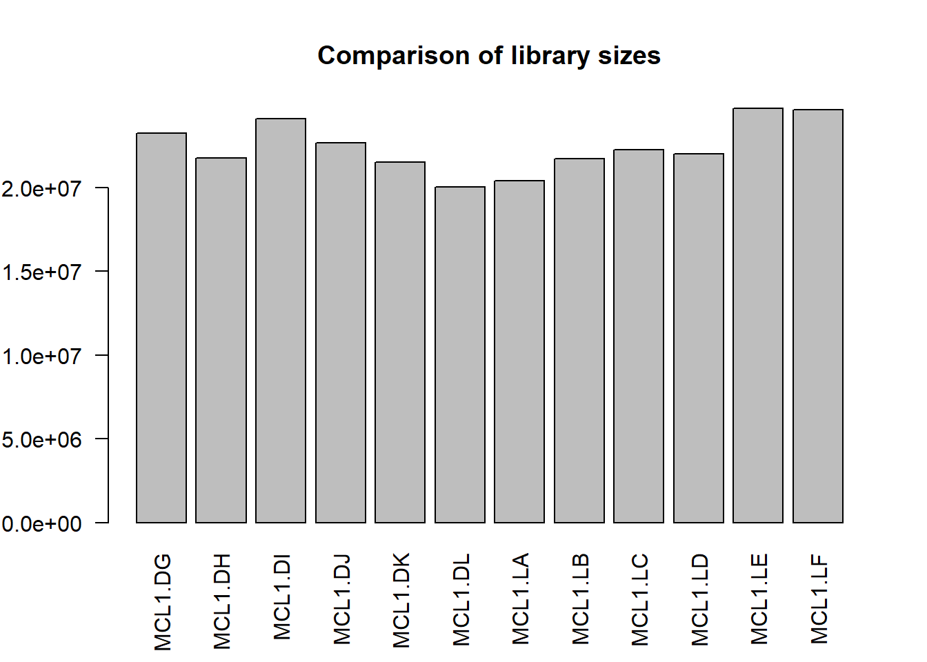
Figure 50.1: Sizes of RNAseq libraries for each sample.
Here’s a plot of the raw counts for each gene, in order to illustrate they are not normally-distributed, which is typical of over-dispersed discrete count data.
boxplot(y$counts, las=2)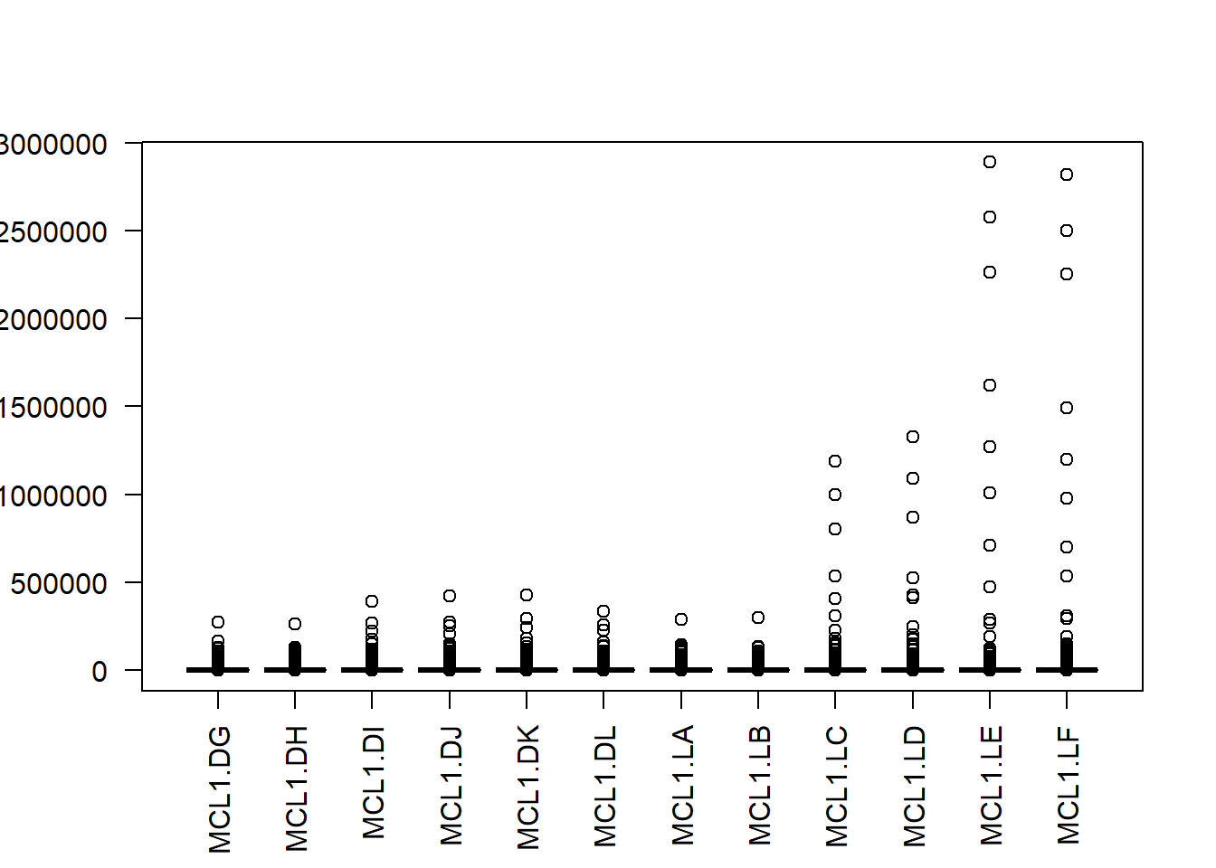
Figure 50.2: Distribution of counts across the 12 samples. Note they are not normally-distributed.
Here’s plot of the data as on-the-fly normalized to CPM, which is also not normally distributed. This illustrates that CPM represents just a simple linear transform of count data.
boxplot(cpm(y$counts), las=2)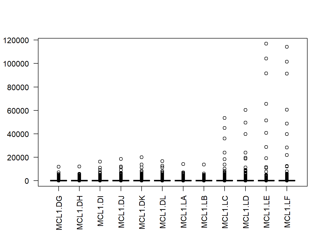
Figure 50.3: Distribution of CPM-transformed counts, still not normally-distributed.
Now let’s plot a log transformation of CPM data. This transformation yields an approximately Gaussian distribution of the count values within each sample, though there are clearly outliers.
The log transformed CPM data will be used in a lot of the statistical modeling below because of this Gaussian property. So we’ll go ahead and make an object for that.
First, we’ll make a log-transformed object.
# Get log2 counts per million. see ?cpm
logcounts <- cpm(y,log=TRUE)
Now look at the logcount date by plotting box plots.
# Check distributions of samples using boxplots
boxplot(logcounts, xlab="", ylab="Log2 counts per million",las=2)
# Let's add a blue horizontal line that corresponds to the median logCPM
abline(h=median(logcounts),col="blue")
title("Boxplots of logCPMs (unnormalised for length)")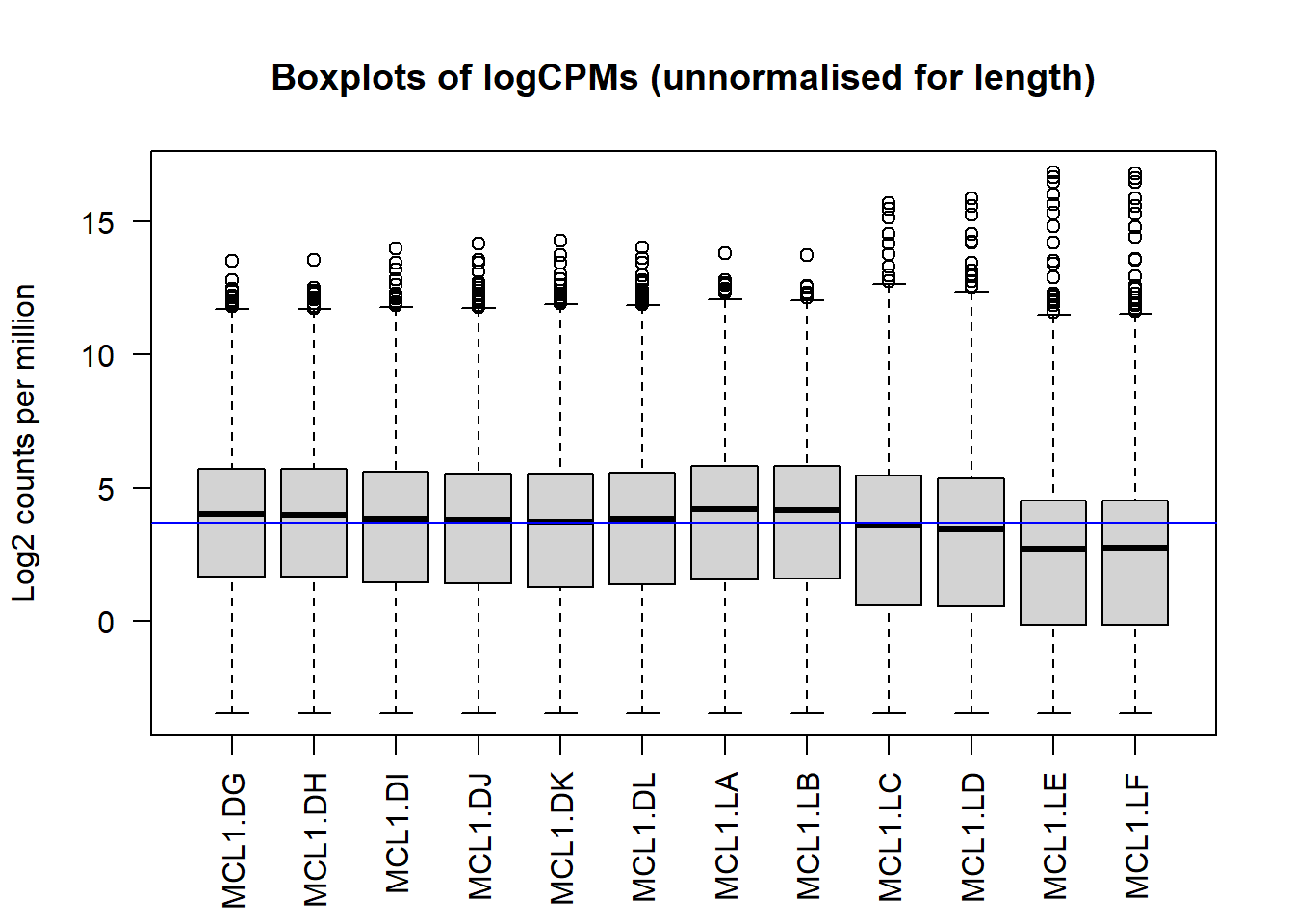
Figure 50.4: Natural log transformed CPM counts, normally-distributed but some outliers.
50.8 Classification
Now, at last, let’s do some statistical modeling.
Multidimensional scaling is a cousin of principal component analysis. It provides a simple way to see if sample groups separate along their first and second dimensions. This is based upon a leading fold-change metric.
This examines the subset of genes that exhibit the largest fold-differences between samples.
The graph below shows separation and clustering of the 12 samples, but it is a bit hard to see what is what this shows us unless you’ve remembered what each sample represents.
limma::plotMDS(y)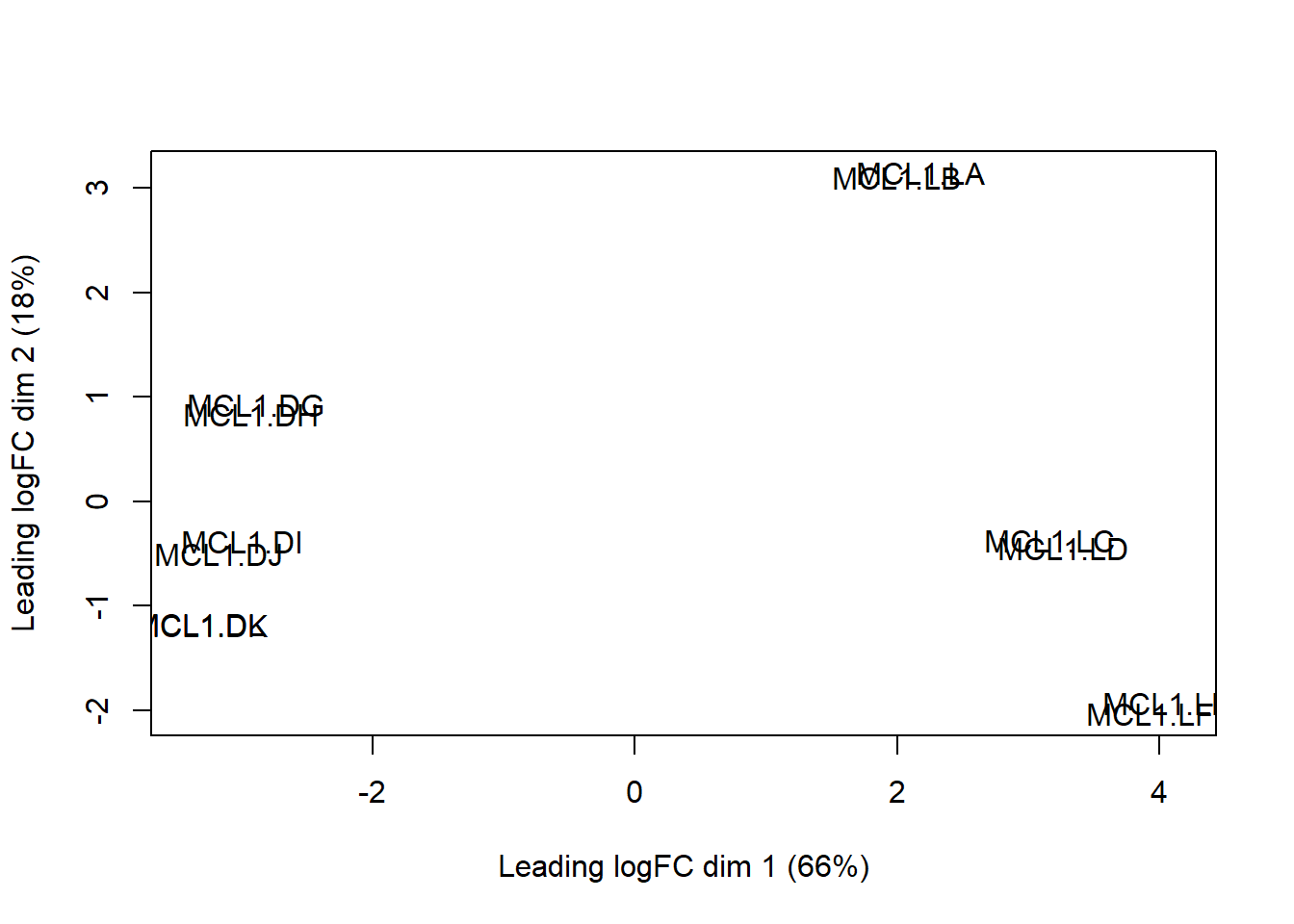
Figure 50.5: Multi-dimensional scaling, a form of PCA.
We’ll munge out some better plots below using color, focusing on the the classification of the predictor variables.
Recall there are 12 samples, duplicates of gene expression in basal and luminal cells, for each of the following three conditions: the cells were derived from mice that were virgin, pregnant, or lactating.
Recall the object sampleinfo from way back at the beginning of this exercise, when we read in the 2nd of two data files?
Let’s remind ourselves what’s in it.
head(sampleinfo, n=8)## FileName SampleName CellType Status
## 1 MCL1.DG_BC2CTUACXX_ACTTGA_L002_R1 MCL1.DG basal virgin
## 2 MCL1.DH_BC2CTUACXX_CAGATC_L002_R1 MCL1.DH basal virgin
## 3 MCL1.DI_BC2CTUACXX_ACAGTG_L002_R1 MCL1.DI basal pregnant
## 4 MCL1.DJ_BC2CTUACXX_CGATGT_L002_R1 MCL1.DJ basal pregnant
## 5 MCL1.DK_BC2CTUACXX_TTAGGC_L002_R1 MCL1.DK basal lactate
## 6 MCL1.DL_BC2CTUACXX_ATCACG_L002_R1 MCL1.DL basal lactate
## 7 MCL1.LA_BC2CTUACXX_GATCAG_L001_R1 MCL1.LA luminal virgin
## 8 MCL1.LB_BC2CTUACXX_TGACCA_L001_R1 MCL1.LB luminal virginFirst we’ll color by the feature that involves basal and luminal.
# Let's set up color schemes for CellType
# How many cell types and in what order are they stored?
levels(as.factor(sampleinfo$CellType))
## [1] "basal" "luminal"We’ll create a color scheme for these two levels of the cell type factor, using our favorite Emory brand colors. The second line in the script below just checks to make sure the col.cell vector was created properly in the first line.
col.cell <- c("#012169","#b58500")[as.factor(sampleinfo$CellType)]
data.frame(sampleinfo$CellType,col.cell)
## sampleinfo.CellType col.cell
## 1 basal #012169
## 2 basal #012169
## 3 basal #012169
## 4 basal #012169
## 5 basal #012169
## 6 basal #012169
## 7 luminal #b58500
## 8 luminal #b58500
## 9 luminal #b58500
## 10 luminal #b58500
## 11 luminal #b58500
## 12 luminal #b58500Now we just add that color scheme for cell type to the MDS plot.
Multidimensional scaling detects the largest sources of variation. In this case, it detects the variation associated with the genes showing the largest fold-differences between cell types.
The plot below, therefore, clearly illustrates that genes that are responsible for the basal/luminal feature represents the first dimension of separation between the samples.
In other words, we can say that the differences between basal and luminal cell gene expression accounts for most of the variation in the set. There are signals in the RNAseq data that separate the two cell types.
# Redo the MDS with cell type color
plotMDS(y,col=col.cell)
# Let's add a legend to the plot so we know which colors correspond to which cell type
legend("topleft",
       fill=c("#012169","#b58500"),legend=levels(as.factor(sampleinfo$CellType)))
# Add a title
title("Cell type")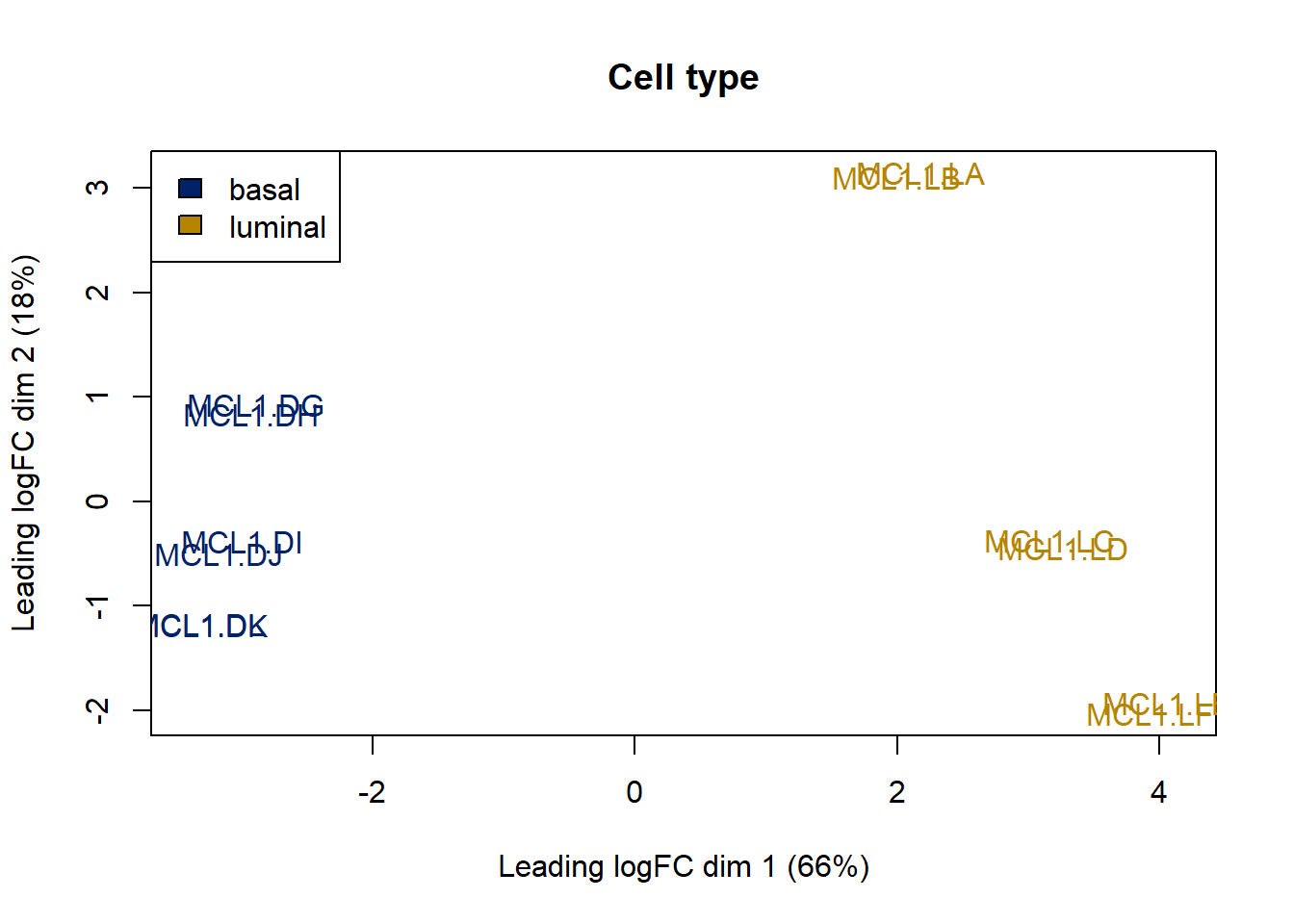
Figure 50.6: MDS shows variation due to cell type explains the first dimension of the data.
Now we’ll do the same coloring trick for the Status variable.
First, what is status?
levels(as.factor(sampleinfo$Status))## [1] "lactate" "pregnant" "virgin"Of course, from each of those three endocrine status, the researchers collected two samples each of basal and luminal cells.
#running out of color imagination
col.status <- c("red","blue","green")[as.factor(sampleinfo$Status)]
col.status
## [1] "green" "green" "blue" "blue" "red" "red" "green" "green" "blue"
## [10] "blue" "red" "red"#just checking how this color coded
head(data.frame(sampleinfo$Status, col.status))## sampleinfo.Status col.status
## 1 virgin green
## 2 virgin green
## 3 pregnant blue
## 4 pregnant blue
## 5 lactate red
## 6 lactate redThe plot below now colors each sample on the basis of whether it is from a virgin, pregnant, or lactating mouse.
There is some separation of them along the 2nd dimension. Note how the duplicates of the same condition are very similar (the MCL1.DL and MCL1.DK are printed on top of each other).
plotMDS(y,col=col.status)
legend("topleft",fill=c("red","blue","green"),
       legend=levels(as.factor(sampleinfo$Status)),cex=0.8)
title("Status")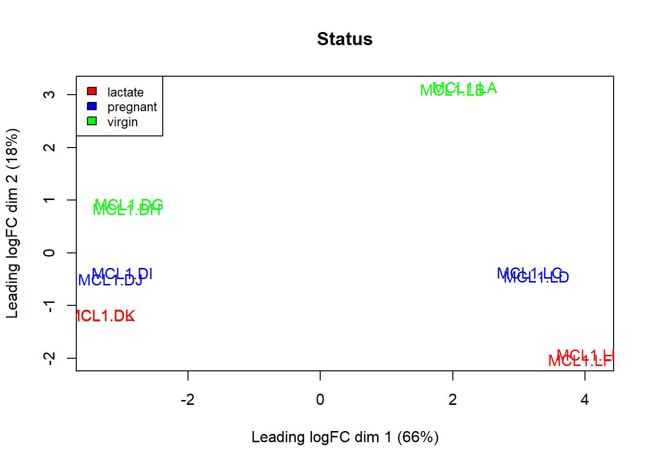
Figure 50.7: Variation due to status represents the 2nd dimension of the data set.
Thus, the greatest dimension of variation of gene expression separates on the basis of cell type, while the second greatest dimension of variation separates on the basis of endocrine status.
Although these dimensions are latent, it is possible to explain what variables are most responsible for the observed variation, and thus explain the first two principal components. The variables here are well chosen: cell type and endocrine status. It’s really a lovely result.
The Bioconductor package PCAtoolsis a veritable smorgasbord of PCA functions and visualizations. Learning this package is strongly recommended. For more on it, see this vignette
50.9 Hierarchical clustering
Hierarchical clustering is a way to cluster while visualizing specific gene relationships to other clusters.
Before illustrating this technique some processing is in order.
We’re interested in seeing the genes driving the dimensional pattern seen above. What genes differ between the two cell types? What genes differ between the 3 status conditions? Is there an interaction between cell type and status?
The most useful approach to answer these kinds of questions would be to focus on the genes that have the highest expression variance across the 12 samples.
Rather than cluster all 15000+ genes, which mostly just adds noise to the analysis, we’ll cluster the 500 that are most variable. This is an arbitrary cutoff, and one that can be played with.
This script creates a vector of variances associated with each GeneID. Just like in ANOVA, when row variances are high, we have a sign the differences between grouping factors will be greatest.
This function simply calculates the variance in the logcounts data frame, row by row. It’s just a numeric vector of variance values that retains the GeneID property.
var_genes <- apply(logcounts, 1, var)
head(var_genes)
## 497097 20671 27395 18777 21399 58175
## 13.6624115 2.7493077 0.1581944 0.1306781 0.3929526 4.8232522class(var_genes)## [1] "numeric"Now produce a character vector with the GeneID names for those that have the greatest to lower variances. In this example, we’ll do up the top 50.
It can be instructive to change this number after viewing a heatmap to lower or higher values.
# Get the gene names for the top 500 most variable genes
select_var <- names(sort(var_genes, decreasing=TRUE))[1:50]
head(select_var)
## [1] "22373" "12797" "11475" "11468" "14663" "24117"class(select_var)## [1] "character"For your information, here is the expression pattern for the GeneID “22373” with the greatest variance. It encodes Wap…. a known regulator of mammary epithelium!
There is much lower expression of Wap in virgin basal cells compared to the others. This passes the bloody obvious test, so long as you remember these are log counts.
logcounts["22373",]## MCL1.DG MCL1.DH MCL1.DI MCL1.DJ MCL1.DK MCL1.DL MCL1.LA
## 0.4660671 0.9113837 7.4350797 7.8078998 9.2883180 9.3184826 6.6277452
## MCL1.LB MCL1.LC MCL1.LD MCL1.LE MCL1.LF
## 6.6884102 12.1273320 13.1502579 15.6481000 15.5696858From logcounts we next select the rows corresponding to these 500 most variable genes.
# Subset logcounts matrix
highly_variable_lcpm <- logcounts[select_var,]
dim(highly_variable_lcpm)
## [1] 50 12head(highly_variable_lcpm)## MCL1.DG MCL1.DH MCL1.DI MCL1.DJ MCL1.DK MCL1.DL MCL1.LA
## 22373 0.4660671 0.9113837 7.435080 7.807900 9.288318 9.318483 6.6277452
## 12797 10.0429713 9.6977966 11.046567 11.358857 11.605894 11.491773 0.8529774
## 11475 12.3849005 12.3247093 13.989573 14.180048 14.285489 14.032486 3.4823396
## 11468 7.1537287 6.8917703 9.325436 9.661942 9.491765 9.424803 -1.8086076
## 14663 1.9717614 1.9471846 9.091895 8.756261 9.539747 9.504098 6.1710357
## 24117 7.8378853 7.8995788 8.634622 8.582447 6.704706 6.777335 -1.3824015
## MCL1.LB MCL1.LC MCL1.LD MCL1.LE MCL1.LF
## 22373 6.6884102 12.1273320 13.1502579 15.6481000 15.569686
## 12797 1.6034598 2.3323371 2.4601069 0.8055694 1.288003
## 11475 4.3708241 5.2116574 5.0788442 3.6997655 3.965775
## 11468 -0.6387584 0.5244769 0.6694047 -0.4412496 -1.014878
## 14663 6.2328260 13.7571928 14.2506761 16.0020840 15.885390
## 24117 -0.5387838 -0.2280797 0.1243601 -2.9468278 -2.945610Creating the hierarchical cluster is now almost anticlimactic.
Now we simply pass this select group of the 500 most variable genes into the heatmap.2 function.
The values represented here are logCPM values.
# Plot the heatmap
heatmap.2(highly_variable_lcpm,
col=viridis,
trace="none",
main="Top variable genes",
scale="row")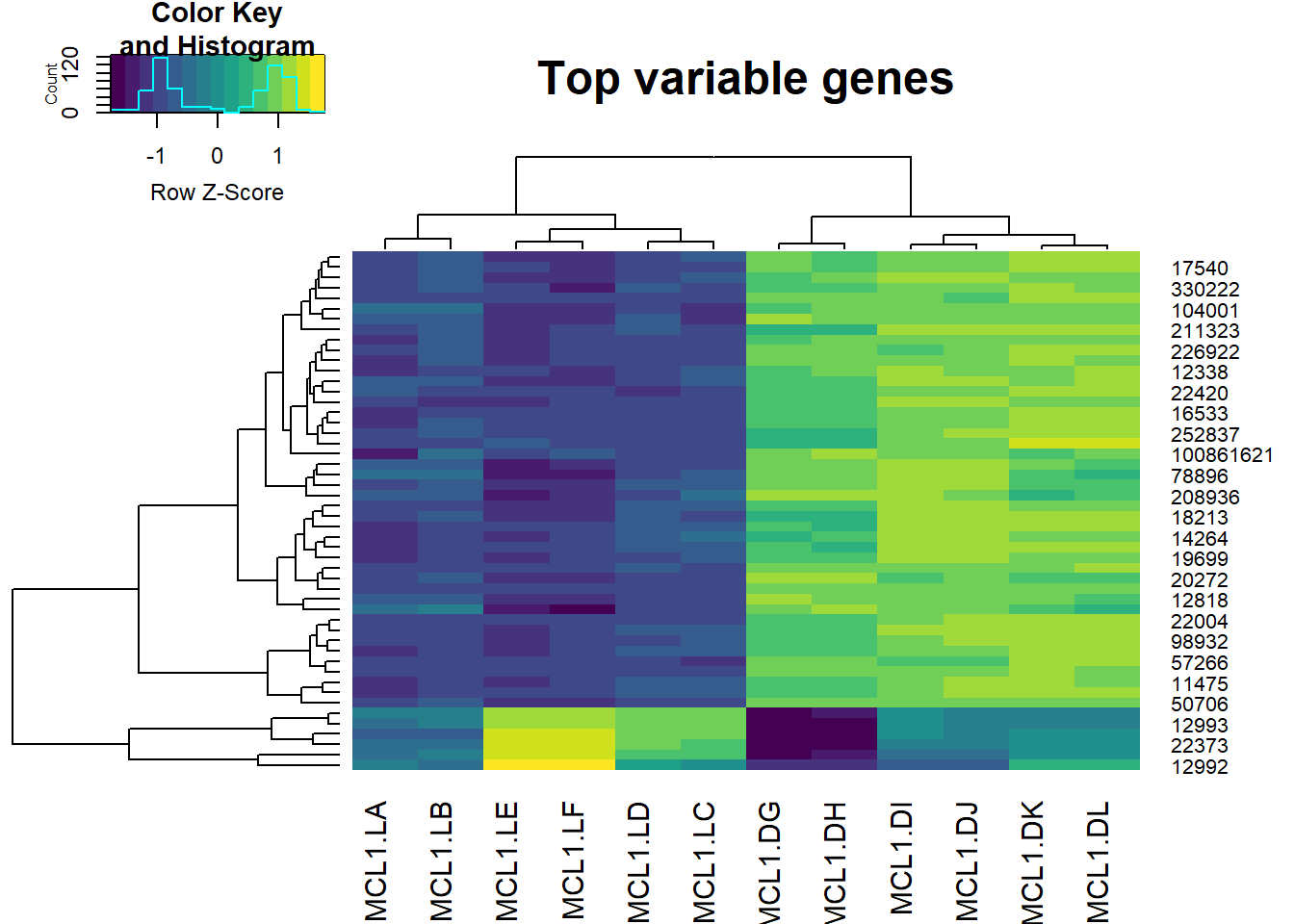 Expression varies from low (dark) to high (light).
Inspection of the horizontal clustering illustrates how it picks up the the experimental design very well. There are two main groups (corresponding to the luminal and basal cell types). There are also 3 groups within each of these, corresponding to the endocrine status.
The endocrine status duplicates line up extremely well together. This is tight data.
The vertical clustering is interesting. Close to 90% of the highly variable genes define the cell type differentiation, while the reminder differentiate the endocrine status (virgin, pregnant, lactating). There is a clear interaction between cell type and status, as well.
50.9.1 Statistical inference on clustering
Some progress has been made to develop an exact test for whether clusters differ. This test does not suffer from the inflated type1 error associated with using standard univariate tests. See the work of Lucy Gao here. Information about her R package clusterpval along with tutorials are here.
50.10 Summary
This chapter is derived from an excellent workshop on using R to work with RNA-seq data. The workshop material is an excellent starting point for learning how to work with this kind of data.
I’ve only covered a small portion of that material and made just a few very modest changes. My goal is making a gentle introduction to working with the data, keeping a focus on classification (MDS and hierarchical clustering).
Install Bioconductor to use this material. Before doing so, it is important to recognize how Bioconductor relates to R and to CRAN. I strongly recommend installing additional Bioconductor packages using the BiocManager. This workflow becomes more important when the time comes to updating, whether R or Bioconductor.
The fundamental currency of RNA-seq data are transcript counts. To work with them first requires transformation via normalization (such as CPM or RPKM).
Counts are not normally distributed. For many statistical treatments the CPM need further conversion to a Gaussian distribution. Natural log transformation usually gets this done.
Scientific judgment is necessary to limit the scope of the datasets. Working with RNA-seq data demands R skills related to creating and working with a variety of on-the-fly data objects, all while keeping one’s rows and columns copacetic.